By Tijana Zrnic
“Scientific research has changed the world. Now it needs to change itself. – The Economist, 2013
There has been a growing concern about the validity of scientific findings. A multitude of journals, papers and reports have recognized the ever smaller number of replicable scientific studies. In 2016, one of the giants of scientific publishing, Nature, surveyed about 1,500 researchers across many different disciplines, asking for their stand on the status of reproducibility in their area of research. One of the many takeaways to the worrisome results of this survey is the following: 90% of the respondents agreed that there is a reproducibility crisis, and the overall top answer to boosting reproducibility was “better understanding of statistics”. Indeed, many factors contributing to the explosion of irreproducible research stem from the neglect of the fact that statistics is no longer as static as it was in the first half of the 20th century, when statistical hypothesis testing came into prominence as a theoretically rigorous proposal for making valid discoveries with high confidence.
When science first saw the rise of statistical testing, the basic idea was the following: you put forward competing hypotheses about the world, then you collect some data, and finally you use these data to validate your hypotheses. Typically, one was in a situation where they could iterate this three-step process only a few times; data was scarce, and the necessary computations were lengthy. Remember, this is early to mid-20th century we are talking about.
This forerunner of today’s scientific investigations would hardly recognize its own field in 2019. Nowadays, testing is much more dynamic and is performed at a scale larger than ever before. Even within a single institution, thousands of hypotheses are tested in a short time interval, older test results inspire future potential analyses, and scientific exploration oftentimes becomes a never-ending stream of individual hypothesis tests. What enabled this explosion of exploratory research is the high-throughput technologies and large amounts of data that we started seeing only recently, at least relative to the era of statistical thinking.
That said, as in any discipline with well-established and successful foundations, it is difficult to move away from classical paradigms in testing. Much of today’s large-scale investigations still uses tools and techniques which, although powerful and supported by beautiful theory, do not take into account that each test might be just a little piece of a much bigger puzzle of exploratory research. Many disciplines have yet to acquire novel methodology for testing, one that promotes valid inferences at scale and thus limits grandiose publications comprised of irreplicable mirages.
Let us analyze why classical hypothesis testing might lead to many spurious conclusions when the number of tests is large. We do so by elaborating the three main steps of a test: “hypothesize”, “collect data” and “validate”.
In the “hypothesize” step, a well-defined null hypothesis is formulated. For example, this could be “jelly beans do not cause acne”; we will use this as our running example. Notice that the null hypothesis, or simply null, is the opposite of what would be considered a discovery. In short, the null is status quo. Also at the beginning of a test, a false positive rate (FPR) is chosen. This is the maximal allowed probability of making a false discovery, typically chosen around 0.05. In the context of our running example, this means the following: if the null is true, i.e. if jelly beans do not cause acne, we will only have a 5% chance of proclaiming causation between jelly beans and acne.
In a frequentist manner, we assume that there is deterministic ground truth about the null hypothesis. That is, it is either true or not. We will refer to the null hypotheses that are true as true nulls, and to those that are false as non-nulls. In our example, if jelly beans do not cause acne, the null hypothesis is a true null. If it is a non-null, however, we would ideally like to proclaim a discovery.
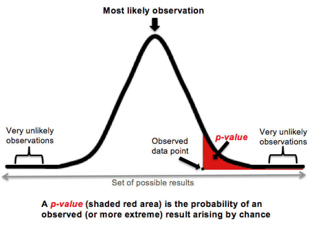
The second step is calculating a p-value based on collected data. This protagonist of many controversies around statistical testing is the probability of seeing the collected data, or something even more extreme, if the null is true. In our example, this is the probability of having some observed parameter of skin condition, or something “even more unusual”, if jelly beans indeed do not cause acne. To illustrate this point, consider the plot below. Let the bell curve be the distribution of the skin parameter if jelly beans do not cause acne. Then, the p-value is the red shaded area under this curve, which is everything “right of” the observed data point. The smaller the p-value, the more unlikely it is that the observation can be explained purely by chance.
The last step is validation. If the calculated p-value is smaller than the FPR, the null hypothesis is rejected, and a discovery is proclaimed. In our running example, if the red shaded area is less than 0.05, we say that jelly beans cause acne.
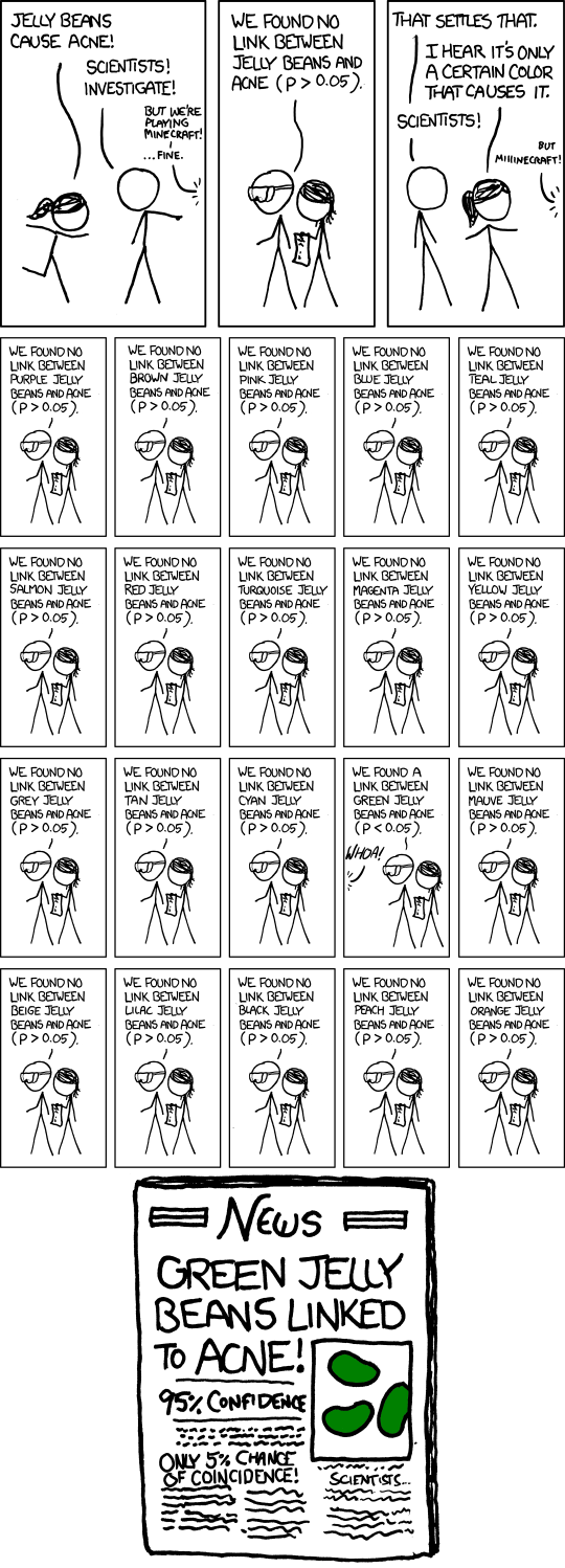
Finally, let us lift the lid on why there are so many false discoveries in large-scale testing. By construction, valid p-values are uniformly distributed on $[0,1]$1, if the null is true. This means that, even if jelly beans do not really cause acne, there is still 0.05 probability that a discovery is falsely proclaimed. Therefore, if testing N hypotheses that are truly null and hence should not be discovered, one is almost certain to proclaim some of them as discoveries if $N$ is large. For example, if all tests are independent, around 5% of $N$ will be discovered. Already after 20 tests of true nulls, even if they are completely arbitrary, one is expected to make a false discovery!
And this is how science goes wrong.
To recap, around 5% of the tested true null hypotheses unfortunately have to be discovered either way, simply by laws of probability. This wouldn’t really be an issue if most of the tested hypotheses were legitimate potential discoveries, i.e. non-nulls. Then, 5% of a small-ish number of true nulls would be negligible. Typically, however, this is not the case. We test loads of crazy, out-there hypotheses, which would attract a lot of attention if confirmed, and we do so simply because we can. In many areas, both observations and computational resources are abundant, so there is little incentive to stay on the “safe side”.
So, how can one make scientific discoveries without the fear of reporting too many false ones?
Controlling the False Discovery Rate
The recognition that a large number of tests leads to almost sure false discoveries has led to various formalisms for controlling their rate of appearance. One powerful proposal, which has become a de facto standard for false discovery control in multiple testing, is called the false discovery rate (FDR), defined as:
Controlling FDR with no additional goal is an easy task; namely, making no discoveries trivially gives FDR = 0. The implict goal behind the vast literature on FDR is discovering as many non-nulls as possible, while keeping FDR controlled under a pre-specified level $\alpha$. We collectively refer to all methods with this goal as FDR methods.
Initially, FDR methods were offline procedures. This means that they required collecting a whole batch of p-values before deciding which tests to proclaim as discoveries. The most notable example of this class is the successful Benjamini-Hochberg procedure, which has for a long time been the default of FDR methods.
However, the scale and scope of modern testing have begun to outstrip this well-recognized methodology. It is far from convenient to wait for all the p-values one wants to test, especially at institutions where testing is a never-ending process. To be more precise, we typically want to make decisions during and between our tests, in particular because this allows us to shape future analyses based on outcomes of past tests. This inspired a new line of work on FDR control, in which decisions are made online.
In online FDR control, p-values arrive one at a time, and the decision of whether or not to make a discovery is made as soon as a p-value is observed. Importantly, online FDR algorithms have enabled controlling FDR over a lifetime; even if the number of sequential tests tends to infinity, one would still have a guarantee that most of the proclaimed discoveries are indeed non-nulls.
The basic principle of online FDR control is to track and control a dynamic quantity called wealth. The wealth represents the current error budget, and is a result of all previously performed tests. In particular, if a test results in a discovery, the wealth increases, while if a discovery is not made, the wealth decreases; note that this update is completely independent of whether the test is truly null or not. When a new test starts, its FPR is chosen based on the available wealth; the bigger the wealth, the bigger the FPR, and consequently the better the chance for a discovery. In fact, this idea has a perfect analogy with testing in a broader social context. To make scientific discoveries, you are awarded an initial grant (corresponding to the target FDR level $\alpha$). This initial funding decreases with every new experiment, and, if you happen to make a scientific discovery, you are again awarded some “wealth”, which you can use toward the budget for subsequent tests. This is essentially the real-world translation of the mathematical expressions guiding online FDR algorithms.
Asynchronous Control of False Discoveries
Although online FDR control has broadened the domain of applications where false discoveries can be controlled, it has failed to account for several important aspects of modern testing.
The main observation is that large-scale testing is not only sequential, but “doubly sequential”. Tests are run in a sequential fashion, but also each test internally is comprised of a sequence of atomic executions, which typically finish at an unpredictable time. This fact makes practitioners run multiple tests that overlap in time in order to gain time efficiency, allowing tests to start and finish at random times.
For example, in clinical trials, it is common to test several different treatment variants against a common control. These trials are often called “perpetual’’, as multiple treatments are tested in parallel, and new treatments enter the testing platform at random times in an online manner. Similarly, A/B testing in industry is typically distributed across many individuals and research teams, and across time, with companies running hundreds of tests per day. This large volume of tests, as well as their complex distribution across many analysts, inevitably causes asynchrony in testing.
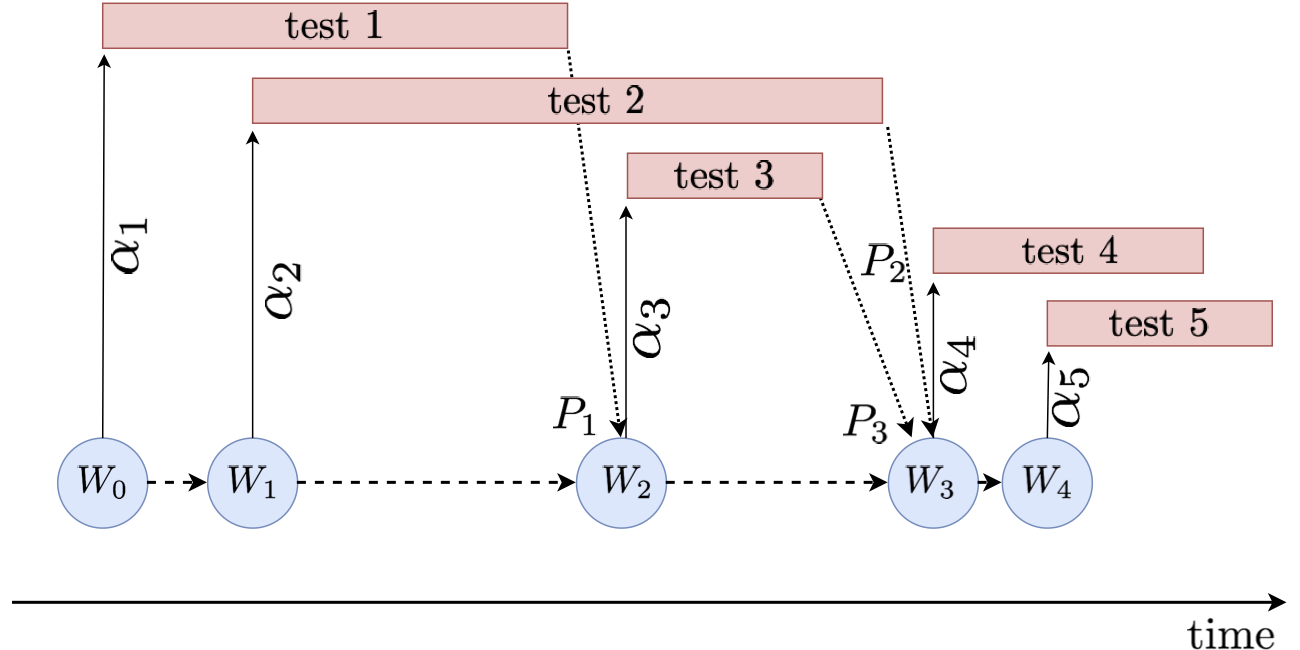
This circumstance is a problem for standard online FDR methodology. Namely, all existing online FDR algorithms assume tests are run synchronously, with no overlap in time; in other words, in order to determine a false positive rate for an upcoming test, online FDR methods need to know the outcomes of all previously started tests. The figure below depicts the difference between synchronous and asynchronous online testing.


For each time step $t$, $W_t$, $P_t$ and $\alpha_t$ are respectively the available wealth at the beginning of the $(t+1)$-th test, the p-value resulting from the $t$-th test, and the FPR of the $t$-th test.
Furthermore, the asynchronous nature of modern testing introduces patterns of dependence between p-values that do not conform to common assumptions. Prior work on online FDR either assumes perfect independence between p-values (overly optimistic), or arbitrary dependence between all tested p-values in the sequence (overly pessimistic). As data are commonly shared across different tests, the first assumption in clearly difficult to satisfy. In clinical trials, having a common control arm induces dependence; in A/B testing, many tests reuse data from the same shared pool, again causing dependence. On the other end, it is not natural to assume that dependence spills over the entire p-value sequence; older data and test outcomes with time become “stale,” and no longer have direct influence on newly created tests. Modern testing calls for an intermediate notion of dependence, called local dependence, one that assumes p-values that are far enough in the sequence are independent, while any two close enough are likely to depend on each other.
In a recent manuscript [1], we developed FDR methods that confront both of these difficulties of large-scale testing. Our methods control FDR in sequential settings that are arbitrarily asynchronous, and/or yield p-values that are locally dependent. Interestingly, from the point of view of our analysis, both local dependence and asynchrony are solved via the same technical instrument, which we call conflict sets. More formally, each new test has a conflict set, which consists of all previously started tests whose outcome is not known (e.g. if there is asynchrony so they are still running), or is known but might have some leverage on the new test (e.g. if there is dependence). We show that computing the FPR of a new test while assuming “unfavorable” outcomes of the conflicting tests is the right approach to guaranteeing FDR control (we call this the principle of pessimism).
It is worth pointing out that FDR control under conflict sets has to be more conservative by construction; to account for dependence between tests, as well as the uncertainty about the tests in progress, the FPRs have to be chosen appropriately smaller. That said, our methods are a strict generalization of prior work on online FDR; they interpolate between standard online FDR algorithms, when the conflict sets are empty, and the Bonferroni correction (also known as alpha-spending), when the conflict sets are arbitrarily large. The latter controls the familywise error rate, which is a more stringent error metric than FDR, under any assumption on how tests relate. This interpolation has introduced the possibility of a tradeoff between the consideration of overall rate of discovery per unit of real time, and consideration of the complexity of careful coordination required to minimize dependence and asynchrony.
Summary
The replicability of hypothesis tests is largely in crisis, as the scale of modern applications has long outstripped classical testing methodology which is still in use. Moreover, prior efforts toward remedying this problem have neglected the fact that testing is massively asynchronous, and hence the existing solutions for boosting reproducibility have not been suitable for many common large-scale testing schemes. Motivated by this observation, we developed methods that control the false discovery rate in complex asynchronous scenarios, allowing statisticians to perform hypothesis tests with a small fraction of false discoveries, and with minimal explicit coordination between tests.
This article was initially published on the BAIR blog, and appears here with the authors’ permission.
References
[1] Zrnic, T., Ramdas, A., & Jordan, M. I. (2018). Asynchronous Online Testing of Multiple Hypotheses. arXiv preprint arXiv:1812.05068.
-
Valid p-values can also be stochastically larger than uniform, which is a more general condition. For simplicity, we take them to be uniform in this text; the “punchline” remains the same either way. ↩

