All posts by Sebastian Castro

An updated guide to Docker and ROS 2

2 years ago, I wrote A Guide to Docker and ROS, which is one of my most frequently viewed posts — likely because it is a tricky topic and people were seeking answers. Since then, I’ve had the chance to use Docker more in my work and have picked up some new tricks. This was long overdue, but I’ve finally collected my updated learnings in this post.

Recently, I encountered an article titled ROS Docker; 6 reasons why they are not a good fit, and I largely agree with it. However, the reality is that it’s still quite difficult to ensure a reproducible ROS environment for people who haven’t spent years fighting the ROS learning curve and are adept at debugging dependency and/or build errors… so Docker is still very much a crutch that we fall back on to get working demos (and sometimes products!) out the door.

If the article above hasn’t completely discouraged you from embarking on this Docker adventure, please enjoy reading.

Revisiting Our Dockerfile with ROS 2

Now that ROS 1 is on its final version and approaching end of life in 2025, I thought it would be appropriate to rehash the TurtleBot3 example repo from the previous post using ROS 2.

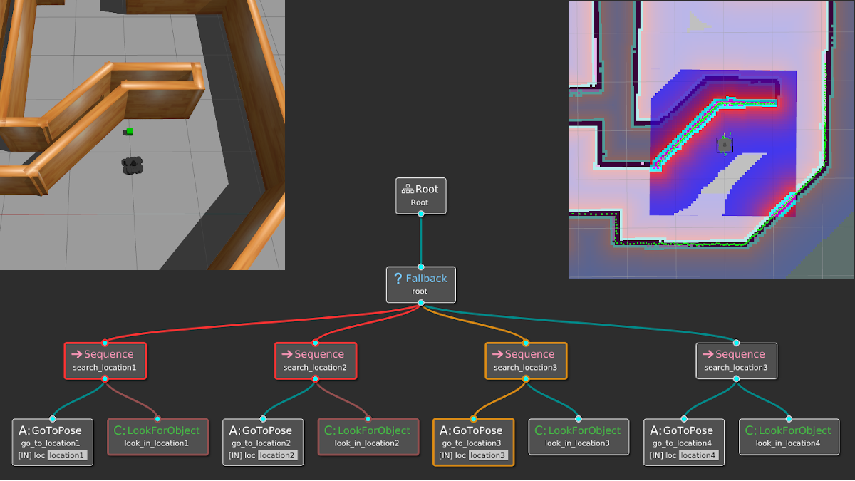
Most of the big changes in this upgrade have to do with ROS 2, including client libraries, launch files, and configuring DDS. The examples themselves have been updated to use the latest tools for behavior trees: BehaviorTree.CPP 4 / Groot 2 for C++ and py_trees / py_trees_ros_viewer for Python. For more information on the example and/or behavior trees, refer to my Introduction to Behavior Trees post.

From a Docker standpoint, there aren’t too many differences. Our container layout will now be as follows:
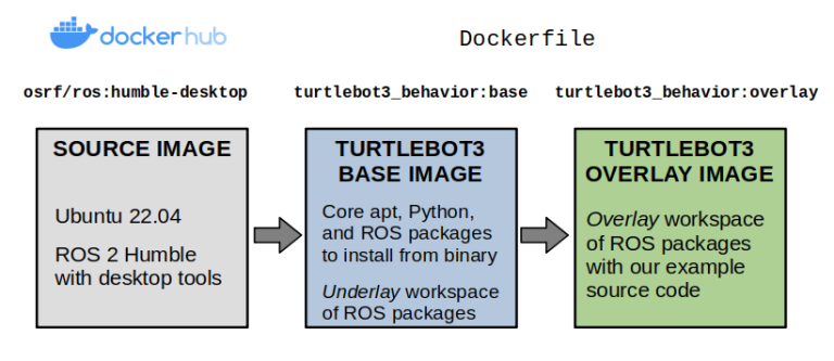
Layers of our TurtleBot3 example Docker image.

We’ll start by making our Dockerfile, which defines the contents of our image. Our initial base layer inherits from one of the public ROS images, osrf/ros:humble-desktop, and sets up the dependencies from our example repository into an underlay workspace. These are defined using a vcstool repos file.

Notice that we’ve set up the argument, ARG ROS_DISTRO=humble, so it can be changed for other distributions of ROS 2 (Iron, Rolling, etc.). Rather than creating multiple Dockerfiles for different configurations, you should try using build arguments like these as much as possible without being “overly clever” in a way that impacts readability.

ARG ROS_DISTRO=humble

########################################
# Base Image for TurtleBot3 Simulation #
########################################
FROM osrf/ros:${ROS_DISTRO}-desktop as base
ENV ROS_DISTRO=${ROS_DISTRO}
SHELL ["/bin/bash", "-c"]

# Create Colcon workspace with external dependencies
RUN mkdir -p /turtlebot3_ws/src
WORKDIR /turtlebot3_ws/src
COPY dependencies.repos .
RUN vcs import < dependencies.repos # Build the base Colcon workspace, installing dependencies first. WORKDIR /turtlebot3_ws RUN source /opt/ros/${ROS_DISTRO}/setup.bash \ && apt-get update -y \ && rosdep install --from-paths src --ignore-src --rosdistro ${ROS_DISTRO} -y \ && colcon build --symlink-install ENV TURTLEBOT3_MODEL=waffle_pi

To build your image with a specific argument — let’s say you want to use ROS 2 Rolling instead — you could do the following… provided that all your references to ${ROS_DISTRO} actually have something that correctly resolves to the rolling distribution.

docker build -f docker/Dockerfile \
--build-arg="ROS_DISTRO=rolling" \
--target base -t turtlebot3_behavior:base .

I personally have had many issues in ROS 2 Humble and later with the default DDS vendor (FastDDS), so I like to switch my default implementation to Cyclone DDS by installing it and setting an environment variable to ensure it is always used.

# Use Cyclone DDS as middleware
RUN apt-get update && apt-get install -y --no-install-recommends \
ros-${ROS_DISTRO}-rmw-cyclonedds-cpp
ENV RMW_IMPLEMENTATION=rmw_cyclonedds_cpp

Now, we will create our overlay layer. Here, we will copy over the example source code, install any missing dependencies with rosdep install, and set up an entrypoint to run every time a container is launched.

###########################################
# Overlay Image for TurtleBot3 Simulation #
###########################################
FROM base AS overlay

# Create an overlay Colcon workspace
RUN mkdir -p /overlay_ws/src
WORKDIR /overlay_ws
COPY ./tb3_autonomy/ ./src/tb3_autonomy/
COPY ./tb3_worlds/ ./src/tb3_worlds/
RUN source /turtlebot3_ws/install/setup.bash \
&& rosdep install --from-paths src --ignore-src --rosdistro ${ROS_DISTRO} -y \
&& colcon build --symlink-install

# Set up the entrypoint
COPY ./docker/entrypoint.sh /
ENTRYPOINT [ "/entrypoint.sh" ]

The entrypoint defined above is a Bash script that sources ROS 2 and any workspaces that are built, and sets up environment variables necessary to run our TurtleBot3 examples. You can use entrypoints to do any other types of setup you might find useful for your application.

#!/bin/bash
# Basic entrypoint for ROS / Colcon Docker containers

# Source ROS 2
source /opt/ros/${ROS_DISTRO}/setup.bash

# Source the base workspace, if built
if [ -f /turtlebot3_ws/install/setup.bash ]
then
source /turtlebot3_ws/install/setup.bash
export TURTLEBOT3_MODEL=waffle_pi
export GAZEBO_MODEL_PATH=$GAZEBO_MODEL_PATH:$(ros2 pkg prefix turtlebot3_gazebo)/share/turtlebot3_gazebo/models
fi

# Source the overlay workspace, if built
if [ -f /overlay_ws/install/setup.bash ]
then
source /overlay_ws/install/setup.bash
export GAZEBO_MODEL_PATH=$GAZEBO_MODEL_PATH:$(ros2 pkg prefix tb3_worlds)/share/tb3_worlds/models
fi

# Execute the command passed into this entrypoint
exec "$@"

At this point, you should be able to build the full Dockerfile:

docker build \
-f docker/Dockerfile --target overlay \
-t turtlebot3_behavior:overlay .

Then, we can start one of our example launch files with the right settings with this mouthful of a command. Most of these environment variables and volumes are needed to have graphics and ROS 2 networking functioning properly from inside our container.

docker run -it --net=host --ipc=host --privileged \
--env="DISPLAY" \
--env="QT_X11_NO_MITSHM=1" \
--volume="/tmp/.X11-unix:/tmp/.X11-unix:rw" \
--volume="${XAUTHORITY}:/root/.Xauthority" \
turtlebot3_behavior:overlay \
bash -c "ros2 launch tb3_worlds tb3_demo_world.launch.py"
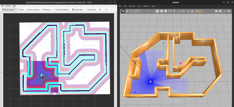
Our TurtleBot3 example simulation with RViz (left) and Gazebo classic (right).

Introducing Docker Compose

From the last few snippets, we can see how the docker build and docker run commands can get really long and unwieldy as we add more options. You can wrap this in several abstractions, including scripting languages and Makefiles… but Docker has already solved this problem through Docker Compose.

In brief, Docker Compose allows you to create a YAML file that captures all the configuration needed to set up building images and running containers.

Docker Compose also differentiates itself from the “plain” Docker command in its ability to orchestrate services. This involves building multiple images or targets within the same image(s) and launching several programs at the same time that comprise an entire application. It also lets you extend existing services to minimize copy-pasting of the same settings in multiple places, define variables, and more.

The end goal is that we have short commands to manage our examples:

  • docker compose build will build what we need
  • docker compose up will launch what we need
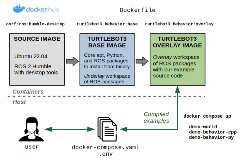
Docker Compose allows us to more easily build and run our containerized examples.

The default name of this magical YAML file is docker-compose.yaml. For our example, the docker-compose.yaml file looks as follows:

version: "3.9"
services:
# Base image containing dependencies.
base:
image: turtlebot3_behavior:base
build:
context: .
dockerfile: docker/Dockerfile
args:
ROS_DISTRO: humble
target: base
# Interactive shell
stdin_open: true
tty: true
# Networking and IPC for ROS 2
network_mode: host
ipc: host
# Needed to display graphical applications
privileged: true
environment:
# Needed to define a TurtleBot3 model type
- TURTLEBOT3_MODEL=${TURTLEBOT3_MODEL:-waffle_pi}
# Allows graphical programs in the container.
- DISPLAY=${DISPLAY}
- QT_X11_NO_MITSHM=1
- NVIDIA_DRIVER_CAPABILITIES=all
volumes:
# Allows graphical programs in the container.
- /tmp/.X11-unix:/tmp/.X11-unix:rw
- ${XAUTHORITY:-$HOME/.Xauthority}:/root/.Xauthority

# Overlay image containing the example source code.
overlay:
extends: base
image: turtlebot3_behavior:overlay
build:
context: .
dockerfile: docker/Dockerfile
target: overlay

# Demo world
demo-world:
extends: overlay
command: ros2 launch tb3_worlds tb3_demo_world.launch.py

# Behavior demo using Python and py_trees
demo-behavior-py:
extends: overlay
command: >
ros2 launch tb3_autonomy tb3_demo_behavior_py.launch.py
tree_type:=${BT_TYPE:?}
enable_vision:=${ENABLE_VISION:?}
target_color:=${TARGET_COLOR:?}

# Behavior demo using C++ and BehaviorTree.CPP
demo-behavior-cpp:
extends: overlay
command: >
ros2 launch tb3_autonomy tb3_demo_behavior_cpp.launch.py
tree_type:=${BT_TYPE:?}
enable_vision:=${ENABLE_VISION:?}
target_color:=${TARGET_COLOR:?}

As you can see from the Docker Compose file above, you can specify variables using the familiar $ operator in Unix based systems. These variables will by default be read from either your host environment or through an environment file (usually called .env). Our example.env file looks like this:

# TurtleBot3 model
TURTLEBOT3_MODEL=waffle_pi

# Behavior tree type: Can be naive or queue.
BT_TYPE=queue

# Set to true to use vision, else false to only do navigation behaviors.
ENABLE_VISION=true

# Target color for vision: Can be red, green, or blue.
TARGET_COLOR=blue

At this point, you can build everything:

# By default, picks up a `docker-compose.yaml` and `.env` file.
docker compose build

# You can also explicitly specify the files
docker compose --file docker-compose.yaml --env-file .env build

Then, you can run the services you care about:

# Bring up the simulation
docker compose up demo-world

# After the simulation has started,
# launch one of these in a separate Terminal
docker compose up demo-behavior-py
docker compose up demo-behavior-cpp
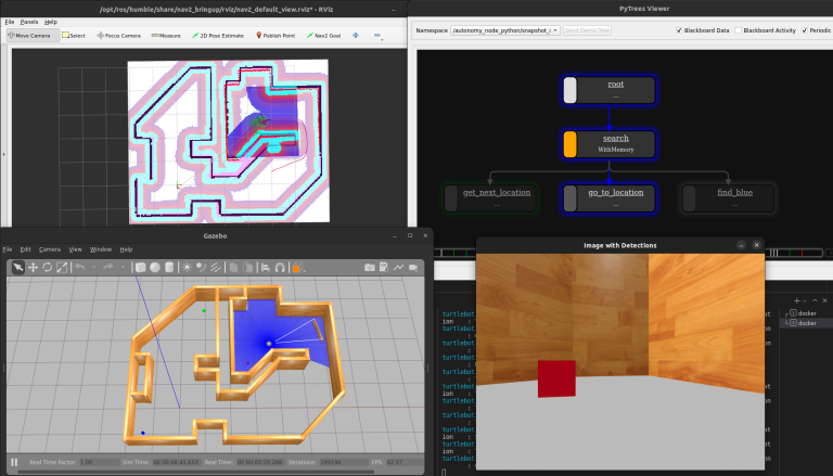
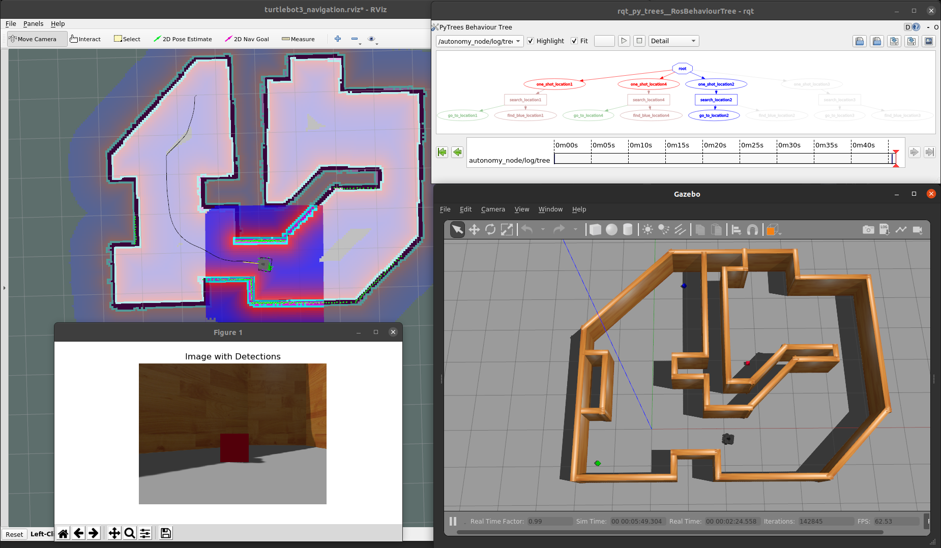
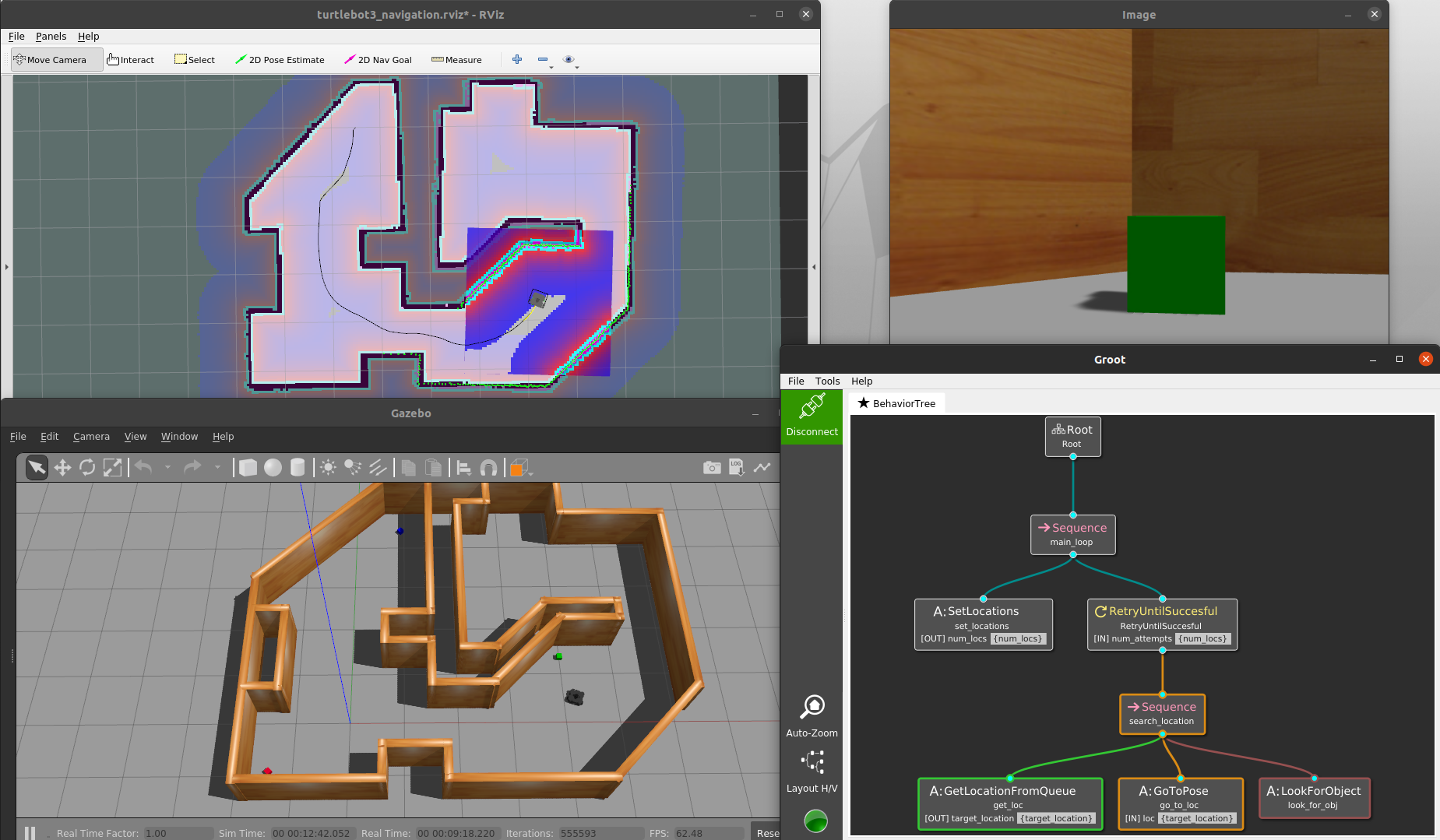
The full TurtleBot3 demo running with py_trees as the Behavior Tree.

Setting up Developer Containers

Our example so far works great if we want to package up working examples to other users. However, if you want to develop the example code within this environment, you will need to overcome the following obstacles:

  • Every time you modify your code, you will need to rebuild the Docker image. This makes it extremely inefficient to get feedback on whether your changes are working as intended. This is already an instant deal-breaker.
  • You can solve the above by using bind mounts to sync up the code on your host machine with that in the container. This gets us on the right track, but you’ll find that any files generated inside the container and mounted on the host will be owned by root as default. You can get around this by whipping out the sudo and chown hammer, but it’s not necessary.
  • All the tools you may use for development, including debuggers, are likely missing inside the container… unless you install them in the Dockerfile, which can bloat the size of your distribution image.

Luckily, there is a concept of a developer container (or dev container). To put it simply, this is a separate container that lets you actually do your development in the same Docker environment you would use to deploy your application.

There are many ways of implementing dev containers. For our example, we will modify the Dockerfile to add a new dev target that extends our existing overlay target.
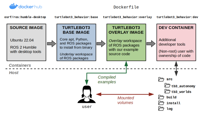
Dev containers allow us to develop inside a container from our host system with minimal overhead.

This dev container will do the following:

  • Install additional packages that we may find helpful for development, such as debuggers, text editors, and graphical developer tools. Critically, these will not be part of the overlay layer that we will ship to end users.
  • Create a new user that has the same user and group identifiers as the user that built the container on the host. This will make it such that all files generated within the container (in folders we care about) have the same ownership settings as if we had created the file on our host. By “folders we care about”, we are referring to the ROS workspace that contains the source code.
  • Put our entrypoint script in the user’s Bash profile (~/.bashrc file). This lets us source our ROS environment not just at container startup, but every time we attach a new interactive shell while our dev container remains up.

#####################
# Development Image #
#####################
FROM overlay as dev

# Dev container arguments
ARG USERNAME=devuser
ARG UID=1000
ARG GID=${UID}

# Install extra tools for development
RUN apt-get update && apt-get install -y --no-install-recommends \
gdb gdbserver nano

# Create new user and home directory
RUN groupadd --gid $GID $USERNAME \
&& useradd --uid ${GID} --gid ${UID} --create-home ${USERNAME} \
&& echo ${USERNAME} ALL=\(root\) NOPASSWD:ALL > /etc/sudoers.d/${USERNAME} \
&& chmod 0440 /etc/sudoers.d/${USERNAME} \
&& mkdir -p /home/${USERNAME} \
&& chown -R ${UID}:${GID} /home/${USERNAME}

# Set the ownership of the overlay workspace to the new user
RUN chown -R ${UID}:${GID} /overlay_ws/

# Set the user and source entrypoint in the user's .bashrc file
USER ${USERNAME}
RUN echo "source /entrypoint.sh" >> /home/${USERNAME}/.bashrc

You can then add a new dev service to the docker-compose.yaml file. Notice that we’re adding the source code as volumes to mount, but we’re also mapping the folders generated by colcon build to a .colcon folder on our host file system. This makes it such that generated build artifacts persist between stopping our dev container and bringing it back up, otherwise we’d have to do a clean rebuild every time.

dev:
extends: overlay
image: turtlebot3_behavior:dev
build:
context: .
dockerfile: docker/Dockerfile
target: dev
args:
- UID=${UID:-1000}
- GID=${UID:-1000}
- USERNAME=${USERNAME:-devuser}
volumes:
# Mount the source code
- ./tb3_autonomy:/overlay_ws/src/tb3_autonomy:rw
- ./tb3_worlds:/overlay_ws/src/tb3_worlds:rw
# Mount colcon build artifacts for faster rebuilds
- ./.colcon/build/:/overlay_ws/build/:rw
- ./.colcon/install/:/overlay_ws/install/:rw
- ./.colcon/log/:/overlay_ws/log/:rw
user: ${USERNAME:-devuser}
command: sleep infinity

At this point you can do:

# Start the dev container
docker compose up dev

# Attach an interactive shell in a separate Terminal
# NOTE: You can do this multiple times!
docker compose exec -it dev bash

Because we have mounted the source code, you can make modifications on your host and rebuild inside the dev container… or you can use handy tools like the Visual Studio Code Containers extension to directly develop inside the container. Up to you.

For example, once you’re inside the container you can build the workspace with:

colcon build

Due to our volume mounts, you’ll see that the contents of the .colcon/build, .colcon/install, and .colcon/log folders in your host have been populated. This means that if you shut down the dev container and bring up a new instance, these files will continue to exist and will speed up rebuilds using colcon build.

Also, because we have gone through the trouble of making a user, you’ll see that these files are not owned by root, so you can delete them if you’d like to clean out the build artifacts. You should try this without making the new user and you’ll run into some annoying permissions roadblocks.

$ ls -al .colcon
total 20
drwxrwxr-x 5 sebastian sebastian 4096 Jul 9 10:15 .
drwxrwxr-x 10 sebastian sebastian 4096 Jul 9 10:15 ..
drwxrwxr-x 4 sebastian sebastian 4096 Jul 9 11:29 build
drwxrwxr-x 4 sebastian sebastian 4096 Jul 9 11:29 install
drwxrwxr-x 5 sebastian sebastian 4096 Jul 9 11:31 log

The concept of dev containers is so widespread at this point that a standard has emerged at containers.dev. I also want to point out some other great resources including Allison Thackston’s blog, Griswald Brooks’ GitHub repo, and the official VSCode dev containers tutorial.

Conclusion

In this post, you have seen how Docker and Docker Compose can help you create reproducible ROS 2 environments. This includes the ability to configure variables at build and run time, as well as creating dev containers to help you develop your code in these environments before distributing it to others.

We’ve only scratched the surface in this post, so make sure you poke around at the resources linked throughout, try out the example repository, and generally stay curious about what else you can do with Docker to make your life (and your users’ lives) easier.

As always, please feel free to reach out with questions and feedback. Docker is a highly configurable tool, so I’m genuinely curious about how this works for you or whether you have approached things differently in your work. I might learn something new!
Integrated Task and Motion Planning (TAMP) in robotics

In the previous post, we introduced task planning in robotics. This field broadly involves a set of planning techniques that are domain-independent: That is, we can design a domain which describes the world at some (typically high) level of abstraction, using some modeling language like PDDL. However, the planning algorithms themselves can be applied to any domain that can be modeled in that language, and critically, to solve any valid problem specification within that domain.

The key takeaway of the last post was that task planning is ultimately search. These search problems are often challenging and grow exponentially with the size of the problem, so it is no surprise that task planning is often symbolic: There are relatively few possible actions to choose from, with a relatively small set of finite parameters. Otherwise, search is prohibitively expensive even in the face of clever algorithms and heuristics.

Bridging the gap between this abstract planning space and the real world, which we deeply care about in robotics, is hard. In our example of a mobile robot navigating a household environment, this might look as follows: Given that we know two rooms are connected, a plan that takes our robot from room A to room B is guaranteed to execute successfully. Of course, this is not necessarily true. We might come up with a perfectly valid abstract plan, but then fail to generate a dynamically feasible motion plan through a narrow hallway, or fail to execute a perfectly valid motion plan on our real robot hardware.

This is where Task and Motion Planning (TAMP) comes in. What if our planner spends more effort deliberating about more concrete aspects of a plan before executing it? This presents a key tradeoff in more up-front computation, but a lower risk of failing at runtime. In this post we will explore a few things that differentiate TAMP from “plain” task planning, and dive into some detailed examples with the pyrobosim and PDDLStream software tools.

Some motivating examples

Before we formalize TAMP further, let’s consider some tricky examples you might encounter with purely symbolic planning in robotics applications.

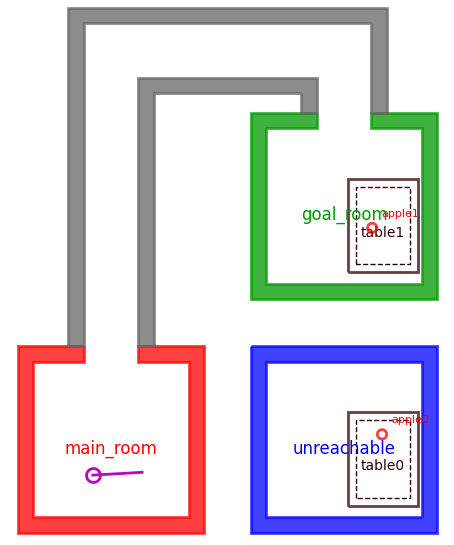
In this first example, our goal is to pick up an apple. In purely symbolic planning where all actions have the same cost, there is no difference in navigating to table0 and table1, both of which have apples. However, you will notice that table0 is in an unreachable location. Furthermore, if we decide to embed navigation actions with a heuristic cost such as straight-line distance from the starting point, our heuristic below will prefer table0 because it’s closer to the robot’s starting position than table1.

It wouldn’t be until we try to refine our plan — for example, using a motion planner to search for a valid path to table0 in the unreachable room — that we would fail, have to update our planning domain to somehow flag that main_room and unreachable are disconnected, and then replan with this new information.

Pathological task planning example for goal-directed navigation.
Both table0 and table1 can lead to solving the goal specification of holding an apple, but table0 is completely unreachable.

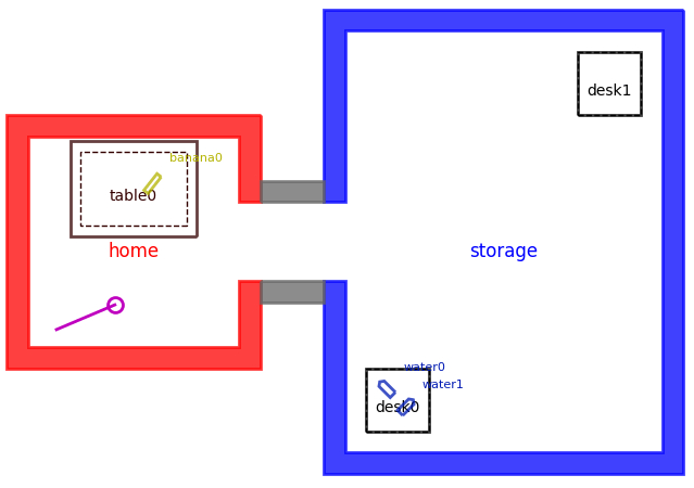
In this second example, we want to place a banana on a desk. As with the previous example, we could choose to place this object on either desk0 or desk1. However, in the absence of more information — and especially if we continue to treat nearby locations as lower cost — we may plan to place banana0 on desk0 and fail to execute at runtime because of the other obstacles.

Here, some alternative solutions would include placing banana0 on desk1, or moving one of the other objects (water0 or water1) out of the way to enable banana0 to fit on desk0. Either way, we need some notion of collision checking to enable our planner to eliminate the seemingly optimal, but in practice infeasible, plan of simply placing the object on desk0.

Pathological task planning example for object manipulation.
Placing banana0 on either desk0 or desk1 will satisfy the goal, but desk0 has other objects that would lead to collisions. So, banana0 must either placed on desk1, or the objects need to be rearranged and/or moved elsewhere to allow banana0 to fit on desk0.

In both cases, what we’re missing from our purely symbolic task planner is the ability to consider the feasibility of abstract actions before spitting out a plan and hoping for the best. Specifically for embodied agents such as robots, which move in the physical world, symbolic plans need to be made concrete through motion planning. As seen in these two examples, what if our task planner also required the existence of a specific path to move between two locations, or a specific pose for placing objects in a cluttered space?

What is Task and Motion Planning?

In our examples, the core issue is that if our task planning domain is too abstract, a seemingly valid plan is likely to fail down the line when we call a completely decoupled motion planner to try execute some portion of that plan. So, task and motion planning is exactly as its name states — jointly thinking about tasks and motion in a single planner. As Garrett et al. put it in their 2020 survey paper, “TAMP actually lies between discrete “high-level” task planning and continuous “low-level” motion planning”.

However, there is no free lunch. When considering all the fine details up front in deliberative planning, search becomes expensive very quickly. In symbolic planning, an action may have a discrete, finite list of possible goals (let’s say somewhere around 5-10), so it may be reasonable to exhaustively search over these and find the one parameter that is optimal according to our model. When we start thinking about detailed motion plans that have a continuous parameter space spanning infinite possible solutions, this becomes intractable. So, several approaches to TAMP will apply sampling-based techniques to make planning work in continuous action spaces.

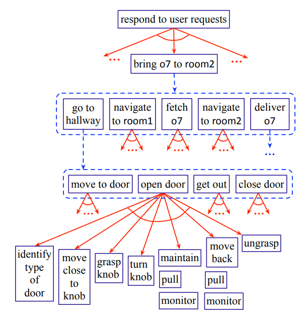
Another way to ensure TAMP is practical is to leverage hierarchy. One popular technique for breaking down symbolic planning into manageable pieces is Hierarchical Task Networks (HTNs). In these 2012 lecture slides, Nilufer Onder mentions “It would be a waste of time to construct plans from individual operators. Using the built-in hierarchy helps escape from exponential explosion.” An example of hierarchical planning is shown in the diagram below. Using this diagram, you can explore the benefits of hierarchy; for example, this planner would never have to even consider how to open a door if the abstract plan didn’t require going down the hallway.

An example of hierarchical planning for a robot, where high-level, or abstract, plans for a robot could be refined into lower-level, or concrete, actions.
Source: Automated Planning and Acting (2016)

Hierarchical planning is great in that it helps prune infeasible plans before spending time producing detailed, low-level plans. However, in this space the mythical downward refinement property is often cited. To directly quote the 1991 paper by Bacchus and Yang, this property states that “given that a concrete-level solution exists, every abstract solution can be refined to a concrete-level solution without backtracking across abstract levels”. This is not always (and I would argue rarely) achievable in robotics, so backtracking in hierarchical planning is largely unavoidable.

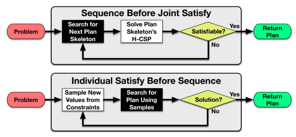
To this end, another strategy behind TAMP has to do with commitment in sampling parameters during search. In the literature, you will see many equivalent words thrown around, but I find the main distinction is between the following strategies:

  • Early-commitment (or binding) strategies will sample action parameters from continuous space before search, effectively converting the problem to a purely discrete task planning problem.
  • Least-commitment (or optimistic) strategies will instead come up with a purely symbolic plan skeleton. If that skeleton is feasible, then the necessary parameter placeholders are filled by sampling.

Flowcharts representing two extreme varieties of sampling-based TAMP.
*H-CSP = hybrid constraint satisfaction problem
Source: Garrett et al. (2020), Integrated Task and Motion Planning

Both strategies have advantages and disadvantages, and in practice modern TAMP methods will combine them in some way that works for the types of planning domains and problems being considered. Also, note that in the diagram above both strategies have a loop back to the beginning when a solution is not found; so backtracking remains an unavoidable part of planning.

One key paper that demonstrated the balance of symbolic search and sampling was Sampling-based Motion and Symbolic Action Planner (SMAP) by Plaku and Hager in 2010. Around the same time, in 2011, Leslie Kaelbling and Tomás Lozano-Pérez presented Hierarchical Planning in the Now (HPN), which combined hierarchy and sampling-based techniques for TAMP. However, the authors themselves admitted the sampling part left something to be desired. There is a great quote in this paper which foreshadows some of the other work that would come out of their lab:

“Because our domains are infinite, we cannot consider all instantiations of the operations. Our current implementation of suggesters only considers a small number of possible instantiations of the operations. We could recover the relatively weak properties of probabilistic completeness by having the suggesters be generators of an infinite stream of samples, and managing the search as a non-deterministic program over those streams.”

– Leslie pack kaelbling and Tomás Lozano-Pérez (2011), Hierarchical planning in the now.

Directly following this quote is the work their student Caelan Garrett took on — first in the creation of STRIPStream in 2017 and then PDDLStream in 2018. The astute reader will have noticed that PDDLStream is the actual software used in these blog posts, so take this “literature review” with this bias in mind, and keep reading if you want to learn more about TAMP with this specific tool.

If you want to know more about TAMP in general, I will refer you to two recent survey papers that I found useful:

Mobile robot example, revisited

To illustrate the benefits of integrated TAMP, we’ll continue the same mobile robotics example from the previous post. In this problem,

  • The robot’s goal is to place the apple on the table.
  • Navigation now requires coming up with a goal pose (which is a continuous parameter), as well the actual path from start to goal. For this example, we are using a Rapidly-exploring Random Tree (RRT), but you could swap for any other path-finding algorithm.
  • Placing an object now requires sampling a valid pose that is inside the placement surface polygon and does not collide with other objects on that surface.

As you read the following list explaining this problem, make sure you scroll through the slideshow below to get a visual representation.

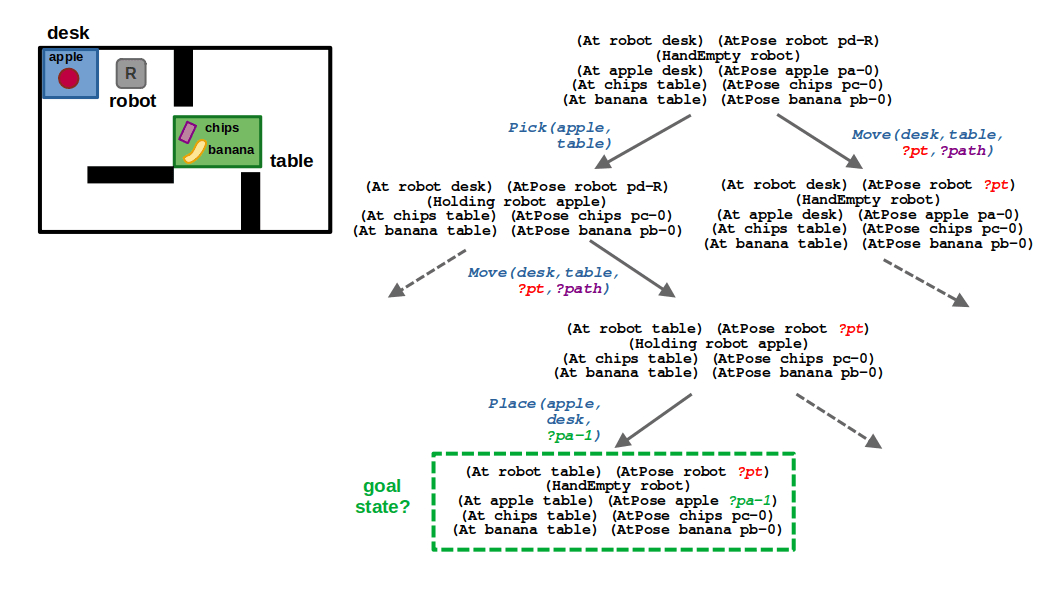
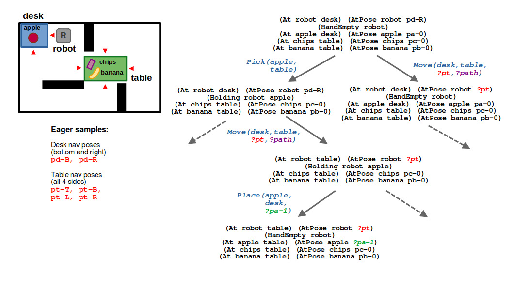
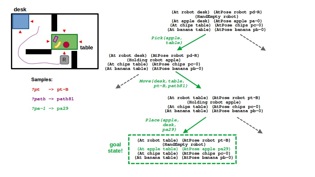
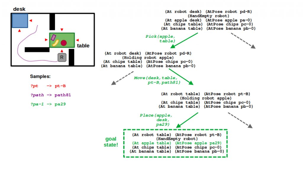
STEP 1: Looking at the state of the world, you can see how a purely symbolic task planner would output a relatively simple plan: pick the apple, move to the table, and place the apple on the table. In the context of TAMP, this now represents a plan skeleton which several parameters that are yet to be filled — specifically,

  • ?pt is the pose of the robot when navigating to the table
  • ?path is the actual output of our motion planner to get to ?pt
  • ?pa-1 is the new pose of the apple when placed on the table (which follows from its initial pose ?pa-0)


STEP 2
: To make the problem a little simpler, we made it such that every location has a discrete, finite set of possible navigation locations corresponding to the edges of its polygon. So looking at the table location, you see there are 4 possible navigation poses pt-T, pt-B, pt-L, and pt-R corresponding to the top, bottom, left, and right sides, respectively. Since this set of locations is relatively small, we can sample these parameters up front (or eagerly) at the start of search.

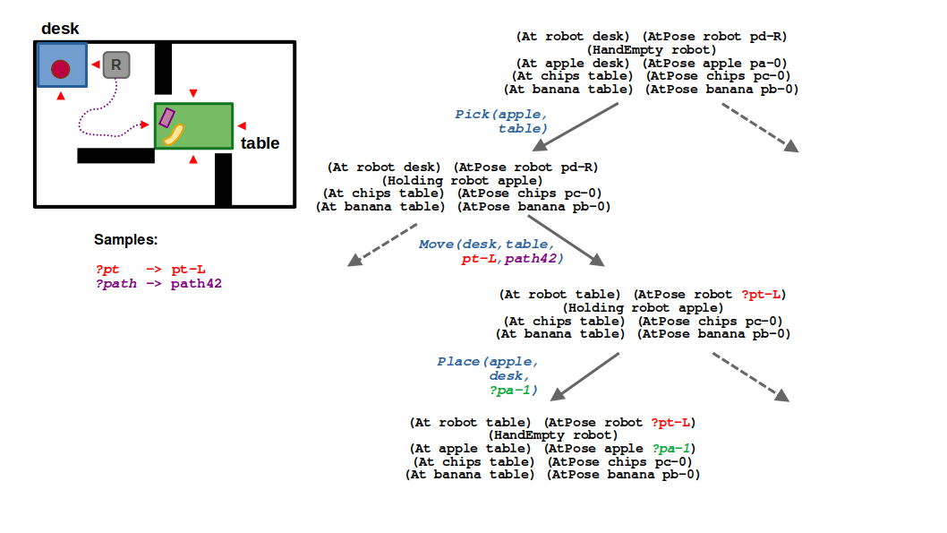
STEP 3: Our move action can now have different instantiations for the goal pose ?pt that are enumerated during search. This is in contrast with the ?path argument, which must be sampled by calling our RRT planner. We don’t want to do this eagerly because the space of paths is continuous, so we prefer to defer sampling of this parameter. If our action has a cost associated with the length of a path, we could imagine that the lowest-cost action would be to navigate to the left side of the table (pt-L), and some randomly sampled path (path42) may describe how we get there.

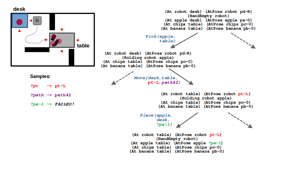
STEP 4: Next comes the place action, which now must include a valid collision-free pose for the apple on the table. Because of how we set up our problem, our robot cannot find a valid placement pose when approaching from the left side of the table. So, we must backtrack.

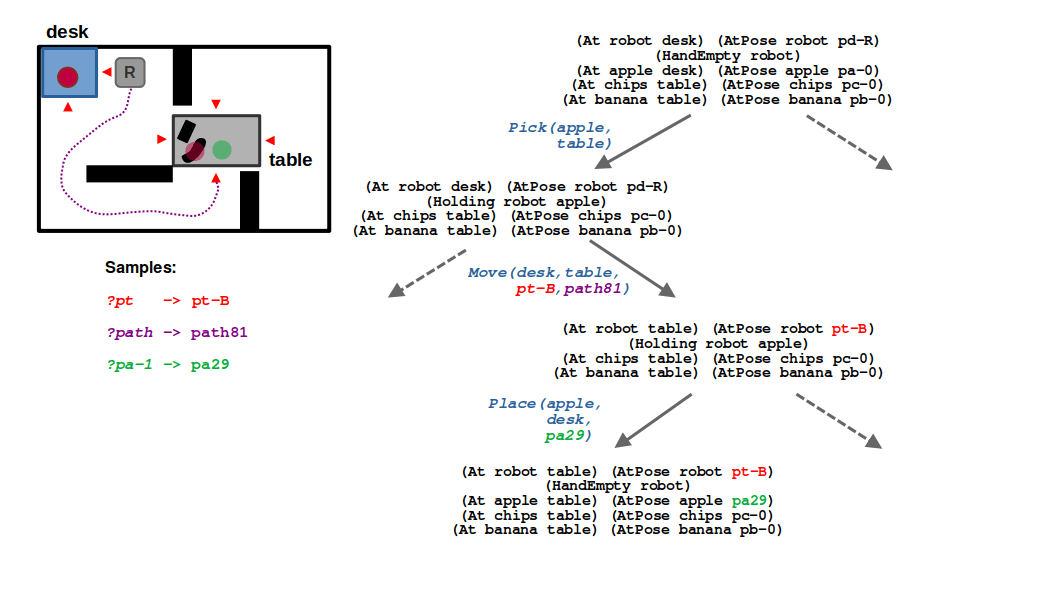
STEP 5: After backtracking, we need to find an alternative navigation pose for the table (?pt). Given our environment, the only other feasible location is the bottom side of the table (pt-b), as the walls block the robot from the top and right sides and it would be impossible to find a valid path with our RRT. However, when the robot is at the bottom side of the table, it can also sample a valid placement pose! In our example, the placeholder ?pa-1 is therefore satisfied with some randomly sampled pose pa29.
STEP 6: … And there you have it! A valid plan that defines a sequence of symbolic actions (pick, move, place) along with the necessary navigation pose, path to that pose, and placement location for the apple. It’s not optimal, but it is probabilistically complete!

(1/6) By being optimistic about all the continuous parameters related to motion, we can reach a potential goal state with relative ease.

(2/6) Since the navigation poses around the desk and the table are finite, we can sample them eagerly; that is, we enumerate all options up front in planning.

(3/6) Once we commit to a navigation pose around the table, we can continue filling in our plan by sampling a feasible trajectory from the robot’s current pose to the target pose at the table.

(4/6) Next, we need to sample a placement pose for the apple. Suppose in this case we fail to sample a collision-free solution based on the robot’s current location.

(5/6) This means we need to backtrack and consider a different navigation pose, thereby a different motion plan to this new pose.

(6/6) From this new pose, even though the trajectory is longer and therefore higher-cost, we can sample a valid placement pose for the apple and finally complete our task and motion plan.

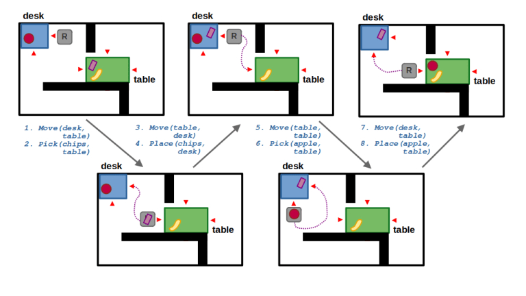
Now, suppose we change our environment such that we can only approach the table from the left side, so there is no way to directly find a valid placement pose for the apple. Using the same planner, we should eventually converge on a task and motion plan that rearranges the objects world — that is, it requires moving one of the other objects on the table to make room for the apple.

Implementing TAMP with PDDLStream

We will now revisit our pathological examples from the beginning of this post. To do this, we will use PDDLStream for planning and pyrobosim as a simple simulation platform. For quick background on PDDLStream, you may refer to this video.

The key idea behind PDDLStream is that it extends PDDL with a notion of streams (remember the earlier quote from the Hierarchical Planning in the Now paper?). Streams are generic, user-defined Python functions that sample continuous parameters such as a valid sample certifies that stream and provides any necessary predicates that (usually) act as preconditions for actions. Also, PDDLStream has an adaptive technique that balances exploration (searching for discrete task plans) vs. exploitation (sampling to fill in continuous parameters).

Goal-directed navigation

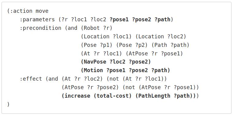
We can use PDDLStream to augment our move action such that it includes metric details about the world. As we saw in our illustrative example, we now must factor in the start and goal pose of our robot, as well as a concrete path between those poses.

As additional preconditions for this action, we must ensure that:

  • The navigation pose is valid given the target location (NavPose)
  • There must be a valid path from the start to goal pose (Motion)

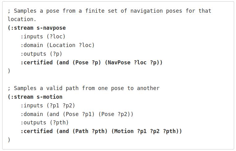
Additionally, we are able to now use more realistic costs for our action by calculating the actual length of our path produced by the RRT! The separate file describing the streams for this action may look as follows. Here, the s-navpose stream certifies the NavPose predicate and the s-motion stream certifies the Motion predicate.

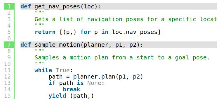
The Python implementations for these functions would then look something like this. Notice that the get_nav_poses function returns a finite set of poses, so the output is a simple Python list. On the other hand, sample_motion can continuously spit out paths from our RRT, and it implemented as a generator:

Putting this new domain and streams together, we can solve our first pathological example from the introduction. In the plan below, the robot will compute a path to the farther away, but reachable room to pick up an apple and satisfy the goal.

Object manipulation

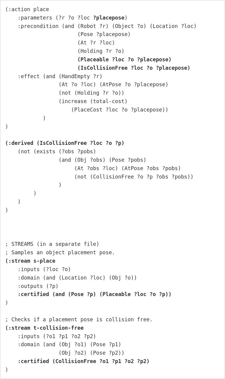
Similarly, we can extend our place action to now include the actual poses of objects in the world. Specifically,

  • The ?placepose argument defines the target pose of the object.
  • The Placeable predicate is certified by a s-place stream.
  • The IsCollisionFree predicate is actually a derived predicate that checks individual collisions between the target object and all other objects at that location.
  • Each individual collision check is determined by the CollisionFree predicate, which is certified by a t-collision-free steam.

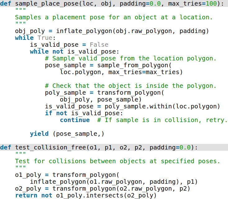
The Python implementation for sampling placement poses and checking for collisions may look as follows. Here, sample_place_pose is our generator for placement poses, whereas test_collision_free is a simple Boolean (true/false) check.

By expanding our domain to reason about the feasibility of object placement, we can similarly solve the second pathological example from the introduction. In the first video, we have an alternative location desk1 where the robot can place the banana and satisfy the goal.

In the second video, we remove the alternative desk1. The same task and motion planner then produces a solution that involves picking up one of the objects on desk0 to make room to later place the banana there.

You can imagine extending this to a more realistic system — that is, one that is not a point robot and has an actual manipulator — that similarly checks the feasibility of a motion plan for picking and placing objects. While it wasn’t the main focus of the work, our Active Learning of Abstract Plan Feasibility work did exactly this with PDDLStream. Specifically, we used RRTs to sample configuration-space paths for a Franka Emika Panda arm and doing collision-checking using a surrogate model in PyBullet!

Conclusion

In this post we introduced the general concept of task and motion planning (TAMP). In theory, it’s great to deliberate more — that is, really think more about the feasibility of plans down to the metric level — but with that comes more planning complexity. However, this can pay off in that it reduces the risk of failing in the middle of executing a plan and having to stop and replan.

We introduced 3 general principles that can make TAMP work in practice:

  • Hierarchy, to determine the feasibility of abstract plans before planning at a lower level of refinement.
  • Continuous parameter spaces, and techniques like sampling to make this tractable.
  • Least-commitment strategies, to come up with symbolic plan skeletons before spending time with expensive sampling of parameters.

We then dug into PDDLStream as one tool for TAMP, which doesn’t do much in the way of hierarchy, but certainly tackles continuous parameter spaces and least-commitment strategies for parameter binding. We went through a few examples using pyrobosim, but you can access the full set of examples in the pyrobosim documentation for TAMP.

The PDDLStream repository has many more examples that you can check out. And, of course, there are many other task and motion planners out there that focus on different things — such as hierarchy without continuous parameters, or factoring in other common objectives such as temporal aspects and resource consumption.

Hope you have enjoyed these posts! If the tools shown here give you any cool ideas, I would love to hear about them, so feel free to reach out.


You can read the original article at Roboticseabass.com.

Task planning in robotics

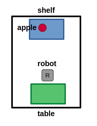
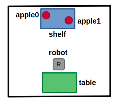
Suppose we have a robot in a simple world like the one below. Let’s consider commanding our robot to perform a task such as “take the apple from the shelf and put it on the table”.

Simple task planning example world: A robot can move between a finite set of locations, and can pick and place objects at those locations.

I would argue we humans have pretty good intuition for how a robot could achieve this task. We could describe what the robot should do by breaking the solution down into individual actions. For example:

  • Move to the shelf
  • Pick up the apple
  • Move back to the table
  • Place the apple

This is fine for our simple example — and in fact, is also fine for many real-world robotics applications — but what if the task gets more complicated? Suppose we add more objects and locations to our simple world, and start describing increasingly complex goals like “make sure all the apples are on the table and everything else is in the garbage bin”? Furthermore, what if we want to achieve this in some optimal manner like minimizing time, or number of total actions? Our reasoning quickly hits its limit as the problem grows, and perhaps we want to consider letting a computer do the work.

This is what we often refer to as task planning: Autonomously reasoning about the state of the world using an internal model and coming up a sequence of actions, or a plan, to achieve a goal.

In my opinion, task planning is not as popular as other areas in robotics you might encounter because… quite frankly, we’re just not that good at robotics yet! What I mean is that robots are complicated, and many commercially available systems are automating simple, repetitive tasks that don’t require this level of high-level planning — it would be overkill! There are many lower-level problems to solve in robotics such as standing up good hardware, robust sensing and actuation, motion planning, and keeping costs down. While task planning skews towards more academic settings for this reason, I eagerly await the not-so-distant future where robots are even more capable and the entire industry is thinking more about planning over longer horizons and increasingly sophisticated tasks.

In this post, I will introduce the basic pieces behind task planning for robotics. I will focus on Planning Domain Definition Language (PDDL) and take you through some basic examples both conceptually and using the pyrobosim tool.

Defining a planning domain

Task planning requires a model of the world and how an autonomous agent can interact with the world. This is usually described using state and actions. Given a particular state of the world, our robot can take some action to transition to another state.

Over the years, there have been several languages used to define domains for task planning. The first task planning language was the STanford Research Institute Problem Solver (STRIPS) in 1971, made popular by the Shakey project.

Since then, several related languages for planning have come up, but one of the most popular today is Planning Domain Definition Language (PDDL). The first PDDL paper was published in 1998, though there have been several enhancements and variations tacked on over the years. To briefly describe PDDL, it’s hard to beat the original paper.

“PDDL is intended to express the “physics” of a domain, that is, what predicates there are, what actions are possible, what the structure of compound actions is, and what the effects of actions are.”

– GHALLAB ET AL. (1998), PDDL – THE PLANNING DOMAIN DEFINITION LANGUAGE

The point of languages like PDDL is that they can describe an entire space of possible problems where a robot can take the same actions, but in different environments and with different goals. As such, the fundamental pieces of task planning with PDDL are a task-agnostic domain and a task-specific problem.

Using our robot example, we can define:

  • Domain: The task-agnostic part
    • Predicates: (Robot ?r), (Object ?o), (Location ?loc), (At ?r ?loc), (Holding ?r ?o), etc.
    • Actions: move(?r ?loc1 ?loc2), pick(?r ?o ?loc), place(?r ?o ?loc)
  • Problem: The task-specific part
    • Objects: (Robot robot), (Location shelf), (Location table), (Object apple)
    • Initial state: (HandEmpty robot), (At robot table), (At apple shelf)
    • Goal specification: (At apple table)

Since domains describe how the world works, predicates and actions have associated parameters, which are denoted by ?, whereas a specific object does not have any special characters to describe it. Some examples to make this concrete:

  • (Location ?loc) is a unary predicate, meaning it has one parameter. In our example, shelf and table are specific location instances, so we say that (Location table) and (Location shelf) are part of our initial state and do not change over time.
  • (At ?r ?loc) is a binary predicate, meaning it has two parameters. In our example, the robot may begin at the table, so we say that (At robot table) is part of our initial state, though it may be negated as the robot moves to another location.

PDDL is an action language, meaning that the bulk of a domain is defined as actions (sometimes referred to as operators) that interact with our predicates above. Specifically, an action contains:

  • Parameters: Allow the same type of action to be executed for different combinations of objects that may exist in our world.
  • Preconditions: Predicates which must be true at a given state to allow taking the action from that state.
  • Effects: Changes in state that occur as a result of executing the action.

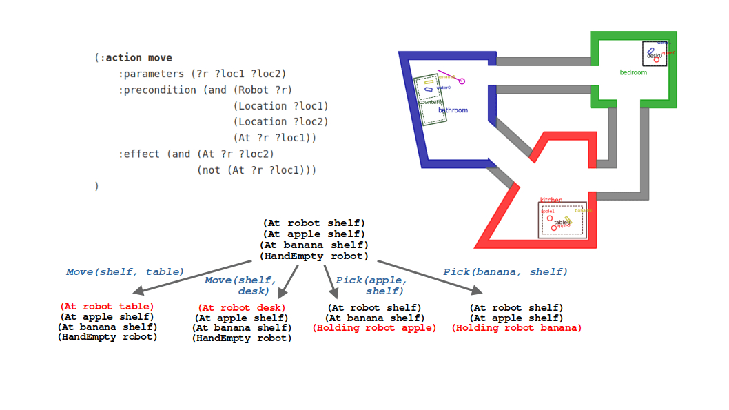
For our robot, we could define a move action as follows:

(:action move
:parameters (?r ?loc1 ?loc2)
:precondition (and (Robot ?r)
(Location ?loc1)
(Location ?loc2)
(At ?r ?loc1))
:effect (and (At ?r ?loc2)
(not (At ?r ?loc1)))
)


In our description of move, we have

  • Three parameters ?r ?loc1, and ?loc2.
  • Unary predicates in the preconditions that narrow down the domain of parameters that make an action feasible — ?r must be a robot and ?loc1 and ?loc2 must be locations, otherwise the action does not make sense.
  • Another precondition that is state-dependent: (At ?r ?loc1). This means that to perform a move action starting at some location ?loc1, the robot must already be in that location.

Note that in some cases, PDDL descriptions allow for typing, which lets you define the domain of actions inline with the parameters rather than explicitly including them as unary predicates — for example, :parameters ?r – Robot ?loc1 – Location ?loc2 – Location … but this is just syntactic sugar.

Similarly, the effects of the action can add new predicates or negate existing ones (in STRIPS these were specified as separate addition and deletion lists). In our example, after performing a move action, the robot is no longer at its previous location ?loc1 and instead is at its intended new location ?loc2.

A similar concept can be applied to other actions, for example pick and place. If you take some time to process the PDDL snippets below, you will hopefully get the gist that our robot can manipulate an object only if it is at the same location as that object, and it is currently not holding something else.

(:action pick
:parameters (?r ?o ?loc)
:precondition (and (Robot ?r)
(Obj ?o)
(Location ?loc)
(HandEmpty ?r)
(At ?r ?loc)
(At ?o ?loc))
:effect (and (Holding ?r ?o)
(not (HandEmpty ?r))
(not (At ?o ?loc)))
)

(:action place
:parameters (?r ?o ?loc)
:precondition (and (Robot ?r)
(Obj ?o)
(Location ?loc)
(At ?r ?loc)
(not (HandEmpty ?r))
(Holding ?r ?o))
:effect (and (HandEmpty ?r)
(At ?o ?loc)
(not (Holding ?r ?o)))
)

So given a PDDL domain, we can now come up a plan, or sequence of actions, to solve various types of problems within that domain … but how is this done in practice?

Task planning is search

There is good reason for all this overhead in defining a planning domain and a good language to express it in: At the end of the day, task planning is solved using search algorithms, and much of the literature is about solving complex problems as efficiently as possible. As task planning problems scale up, computational costs increase at an alarming rate — you will often see PSPACE-Complete and NP-Complete thrown around in the literature, which should make planning people run for the hills.

State-space search

One way to implement task planning is using our model to perform state-space search. Given our problem statement, this could either be:

  • Forward search: Start with the initial state and expand a graph until a goal state is reached.
  • Backward search: Start with the goal state(s) and work backwards until the initial state is reached.

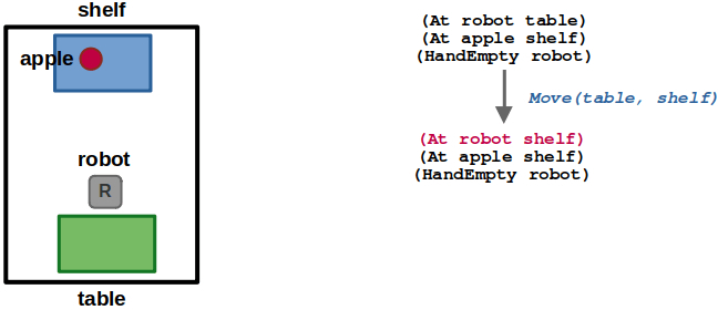
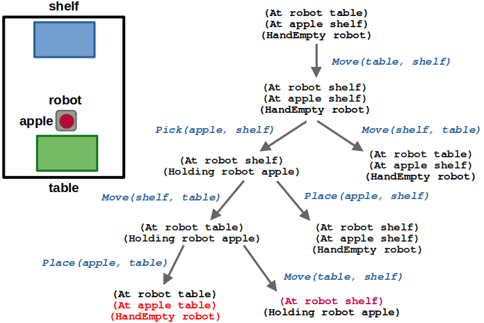
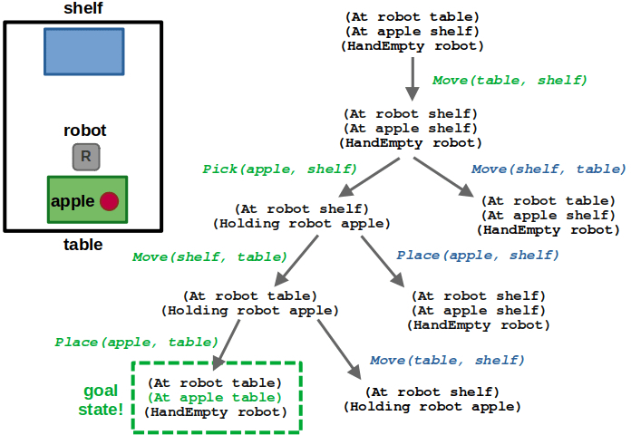
Using our example, let’s see how forward state-space search would work given the goal specification (At apple table):

(1/6) In our simple world, the robot starts at the table. The only valid action from here is to move to the shelf.

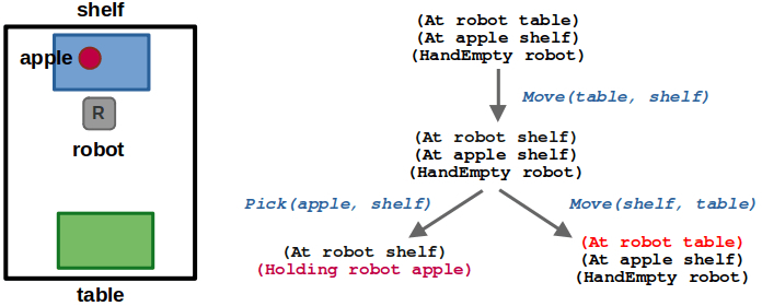
(2/6) After moving to the shelf, the robot could either pick the apple or move back to the table. Since moving back to the table leads us to a state we have already seen, we can ignore it.

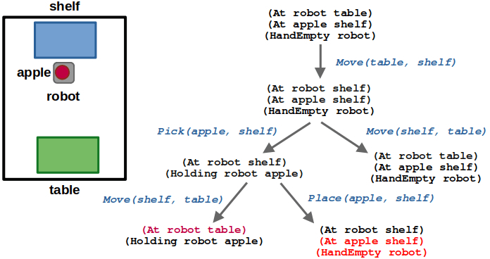
(3/6) After picking the apple, we could move back to the table or place the apple back on the shelf. Again, placing the apple would lead us to an already visited state.

(4/6) Once the robot is at the table while holding the apple, we can place the apple on the table or move back to the shelf.

(5/6) At this point, if we place the apple on the table we reach a goal state! The sequence of actions leading to the state is our resulting plan.

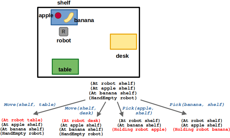
(6/6) As the number of variables increases, the search problem (and time to find a solution) grows exponentially.

Deciding which states to expand during search could be purely based on a predetermined traversal strategy, using standard approaches like breadth-first search (BFS), depth-first search (DFS), and the like. Whether we decide to add costs to actions or treat them all as unit cost (that is, an optimal plan simply minimizes the total number of actions), we could instead decide to use greedy or hill-climbing algorithms to expand the next state based on minimum cost. And finally, regardless of which algorithm we use, we probably want to keep track of states we have already previously visited and prune our search graph to prevent infinite cycles and expanding unnecessary actions.

In motion planning, we often use heuristics during search; one common example is the use of A* with the straight-line distance to a goal as an admissible heuristic. But what is a good heuristic in the context of task planning? How would you define the distance to a goal state without a handy metric like distance? Indeed, a great portion of the literature focuses on just this. Methods like Heuristic Search Planning (HSP) and Fast-Forward (FF) seek to define heuristics by solving relaxed versions of the problem, which includes removing preconditions or negative effects of actions. The de facto standard for state-space search today is a variant of these methods named Fast Downward, whose heuristic relies on building a causal graph to decompose the problem hierarchically — effectively taking the computational hit up front to transform the problem into a handful of approximate but smaller problems that proves itself worthwhile in practice.

Below is an example using pyrobosim and the PDDLStream planning framework, which specifies a more complex goal that uses the predicates we described above. Compared to our example in this post, the video below has a few subtle differences in that there is a separate class of objects to represent the rooms that the robot can navigate, and locations can have multiple placement areas (for example, the counter has separate left and right areas).

  • (At robot bedroom)
  • (At apple0 table0_tabletop)
  • (At banana0 counter0_left)
  • (Holding robot water0)


pyrobosim example showing a plan that sequences navigation, pick, and place actions.

Alternative search methods

While forward state-space search is one of the most common ways to plan, it is not the only one. There are many alternative search methods that seek to build alternate data structures whose goal is to avoid the computational complexity of expanding a full state-transition model as above. Some common methods and terms you will see include:

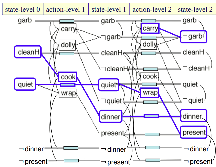
In general, these search methods tend to outperform state-space search in tasks where there are several actions that can be performed in any order relative to each other because they depend on, and affect, mutually exclusive parts of the world. One of the canonical simple examples is the “dinner date example” which is used to demonstrate Graphplan. While these slides describe the problem in more detail, the idea is that a person is preparing a dinner date where the end goal is that dinner and a present be ready while the house is clean — or (dinner present ¬garb). By thinking about the problem in this planning graph structure, we can gain the following insights:

  1. Planning seeks to find actions that can be executed independently because they are mutually exclusive (mutex). This where the notion of partial ordering comes in, and why there are computational gains compared to explicit state-space search: Instead of separately searching through alternate paths where one action occurs before the other, here we simply say that the actions are mutex and we can figure out which to execute first after planning is complete.
  2. This problem cannot be solved at one level because cooking requires clean hands (cleanH) and wrapping the present requires quiet, whereas the two methods of taking out the garbage (carry and dolly) negate these predicates, respectively. So in the solution below, we must expand two levels of the planning graph and then backtrack to get a concrete plan. We first execute cook to remove the requirement on cleanH, and then perform the other two actions in any order — it does not matter.
  3. There is an alternative solution where at the first level we execute the wrap action, and at the second level we can execute cook and dolly (in either order) to achieve the goal. You can imagine this solution would be favored if we additionally required our dinner date hero to have clean hands before starting their date — gross!

Planning graph for the dinner date problem [Source].
Straight lines are preconditions and effects, lines with boxes are no-operation (no-op) links, and curved lines are mutual exclusion (mutex) links.
One solution to the problem is highlighted in blue by backtracking from the goal state.

To bring this all full-circle, you will sometimes find state-space search implementations that use methods like Graphplan on a relaxed version of the problem to estimate the cost to goal as a heuristic. If you want to dig into the details, I would recommend A Tutorial on Planning Graph-Based Reachability Heuristics, by Daniel Bryce and Subbarao Kambhampati.

Towards more complex tasks

Let’s get back to our mobile robot example. What if we want to describe more complex action preconditions and/or goal specifications? After all, we established at the start of this post that simple tasks probably don’t need the giant hammer that is a task planner. For example, instead of requesting that a specific object be placed at a specific location, we could move towards something more general like “all apples should be on the table”.

New example world containing objects, apple0 and apple1, which belong to the same object type (apple).

To explore this, let’s add predicates denoting objects belonging to categories. For example, (Type ?t) can define a specific type and (Is ?o ?t) to denote that an object belongs to such a type. Concretely, we could say that (Type apple), (Is apple0 apple), and (Is apple1 apple).

We can then add a new derived predicate (Has ?loc ?entity) to complete this. Derived predicates are just syntactic sugar — in this case, it helps us to succinctly define an entire space of possible states from our library of existing predicates. However, it lets us express more elaborate ideas in less text. For example:

  • (Has table apple0) is true if the object apple0 is at the location table.
  • (Has table apple) is true if at least one object of type apple is at the location table.

If we choose the goal state (Has table apple) for our example, a solution could involve placing either apple0 or apple1 on the table. One implementation of this derived predicate could look as follows, which makes use of the exists keyword in PDDL.

(:derived (Has ?loc ?entity)
(or
; CASE 1: Entity is a specific object instance, e.g.,
; (Has table apple0)
(and (Location ?loc)
(Obj ?entity)
(At ?entity ?loc)
)
; CASE 2: Entity is a specific object category, e.g.,
; (Has table apple)
(exists (?o)
(and (Obj ?o)
(Location ?loc)
(Type ?entity)
(Is ?o ?entity)
(At ?o ?loc)
)
)
)
)

Another example would be a HasAll derived predicate, which is true if and only if a particular location contains every object of a specific category. In other words, if you planned for (HasAll table apple), you would need both apple0 and apple1 to be relocated. This could look as follows, this time making use of the imply keyword in PDDL.

(:derived (HasAll ?loc ?objtype)
(imply
(and (Obj ?o)
(Type ?objtype)
(Is ?o ?objtype))
(and (Location ?loc)
(At ?o ?loc))
)
)

You could imagine also using derived predicates as preconditions for actions, to similarly add abstraction in other parts of the planning pipeline. Imagine a robot that can take out your trash and recycling. A derived predicate could be useful to allow dumping a container into recycling only if all the objects inside the container are made of recyclable material; if there is any non-recyclable object, then the robot can either pick out the violating object(s) or simply toss the container in the trash.

Below is an example from pyrobosim where we command our robot to achieve the following goal, which now uses derived predicates to express locations and objects either as specific instance, or through their types:

  • (Has desk0_desktop banana0)
  • (Has counter apple1)
  • (HasNone bathroom banana)
  • (HasAll table water)


pyrobosim example showing task planning with derived predicates.

Conclusion

This post barely scratched the surface of task planning, but also introduced several resources where you can find out more. One central resource I would recommend is the Automated Planning and Acting textbook by Malik Ghallab, Dana Nau, and Paolo Traverso.

Some key takeaways are:

  1. Task planning requires a good model and modeling language to let us describe a task-agnostic planning framework that can be applied to several tasks.
  2. Task planning is search, where the output is a plan, or a sequence of actions.
  3. State-space search relies on clever heuristics to work in practice, but there are alternative partial-order methods that aim to make search tractable in a different way.
  4. PDDL is one of the most common languages used in task planning, where a domain is defined as the tool to solve several problems comprising a set of objects, initial state, and goal specification.
  5. PDDL is not the only way to formalize task planning. Here are a few papers I enjoyed:

After reading this post, the following should now make a little more sense: Some of the more recent task planning systems geared towards robotics, such as the ROS2 Planning System (PlanSys2) and PDDLStream, leverage some of these planners mentioned above. Specifically, these use Fast Downward and POPF.

One key pitfall of task planning — at least in how we’ve seen it so far — is that we are operating at a level of abstraction that is not necessarily ideal for real-world tasks. Let’s consider these hypothetical scenarios:

  • If a plan involves navigating between two rooms, but the rooms are not connected or the robot is too large to pass through, how we do know this before we’re actually executing the plan?
  • If a plan involves placing 3 objects on a table, but the objects physically will not fit on that table, how do we account for this? And what if there is some other combination of objects that does fit and does satisfy our goal?

To address these scenarios, there possibly is a way to introduce more expert knowledge to our domain as new predicates to use in action preconditions. Another is to consider a richer space of action parameters that reasons about metric details (e.g., specific poses or paths to a goal) more so than a purely symbolic domain would. In both cases, we are thinking more about action feasibility in task planning. This leads us to the field commonly known as task and motion planning (TAMP), and will be the focus of the next post — so stay tuned!

In the meantime, if you want to explore the mobile robot examples in this post, check out my pyrobosim repository and take a look at the task and motion planning documentation.

Building a python toolbox for robot behavior

If you’ve been subject to my posts on Twitter or LinkedIn, you may have noticed that I’ve done no writing in the last 6 months. Besides the whole… full-time job thing … this is also because at the start of the year I decided to focus on a larger coding project.

At my previous job, I stood up a system for task and motion planning (TAMP) using the Toyota Human Support Robot (HSR). You can learn more in my 2020 recap post. While I’m certainly able to talk about that work, the code itself was closed in two different ways:

  1. Research collaborations with Toyota Research Institute (TRI) pertaining to the HSR are in a closed community, with the exception of some publicly available repositories built around the RoboCup@Home Domestic Standard Platform League (DSPL).
  2. The code not specific to the robot itself was contained in a private repository in my former group’s organization, and furthermore is embedded in a massive monorepo.

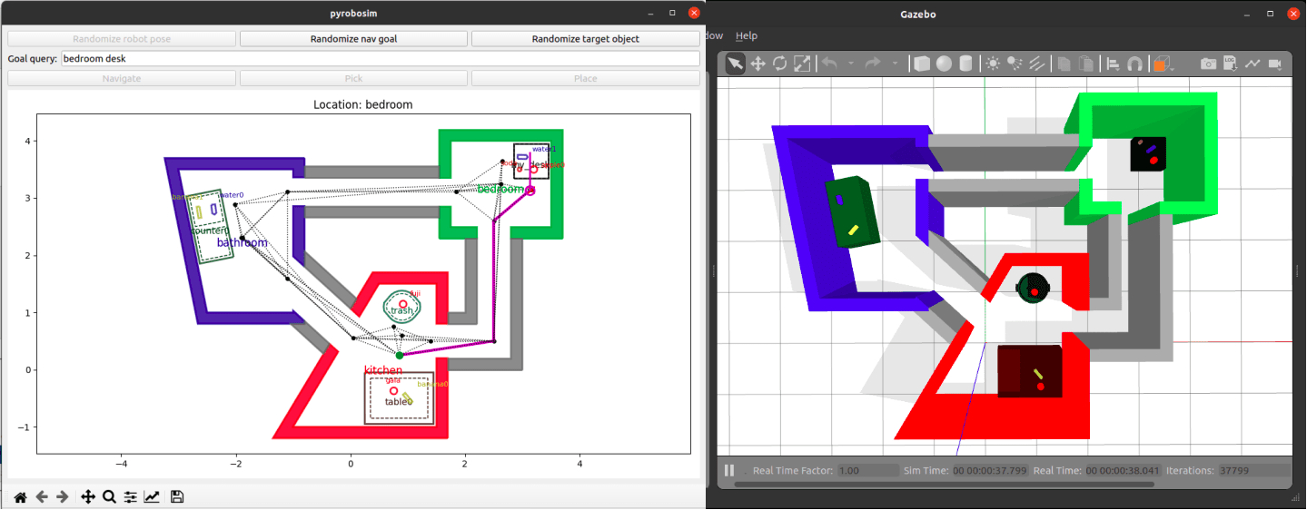
Rewind to 2020: The original simulation tool (left) and a generated Gazebo world with a Toyota HSR (right).

So I thought, there are some generic utilities here that could be useful to the community. What would it take to strip out the home service robotics simulation tools out of that setting and make it available as a standalone package? Also, how could I squeeze in improvements and learn interesting things along the way?

This post describes how these utilities became pyrobosim: A ROS2 enabled 2D mobile robot simulator for behavior prototyping.

What is pyrobosim?

At its core, pyrobosim is a simple robot behavior simulator tailored for household environments, but useful to other applications with similar assumptions: moving, picking, and placing objects in a 2.5D* world.

* For those unfamiliar, 2.5D typically describes a 2D environment with limited access to a third dimension. In the case of pyrobosim, this means all navigation happens in a 2D plane, but manipulation tasks occur at a specific height above the ground plane.

The intended workflow is:

  1. Use pyrobosim to build a world and prototype your behavior
  2. Generate a Gazebo world and run with a higher-fidelity robot model
  3. Run on the real robot!

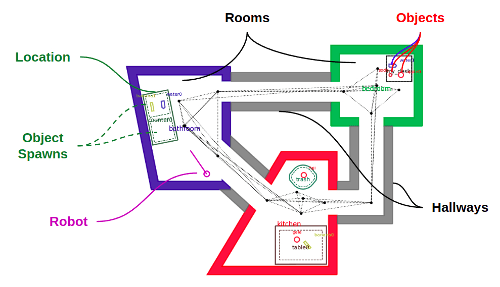
Pyrobosim allows you to define worlds made up of entities. These are:

  • Robots: Programmable agents that can act on the world to change its state.
  • Rooms: Polygonal regions that the robot can navigate, connected by Hallways.
  • Locations: Polygonal regions that the robot cannot drive into, but may contain manipulable objects. Locations contain one of more Object Spawns. This allows having multiple object spawns in a single entity (for example, a left and right countertop).
  • Objects: The things that the robot can move to change the state of the world.

Main entity types shown in a pyrobosim world.

Given a static set of rooms, hallways, and locations, a robot in the world can then take actions to change the state of the world. The main 3 actions implemented are:

  • Pick: Remove an object from a location and hold it.
  • Place: Put a held object at a specific location and pose within that location.
  • Navigate: Plan and execute a path to move the robot from one pose to another.

As this is mainly a mobile robot simulator, there is more focus on navigation vs. manipulation features. While picking and placing are idealized, which is why we can get away with a 2.5D world representation, the idea is that the path planners and path followers can be swapped out to test different navigation capabilities.

Another long-term vision for this tool is that the set of actions itself can be expanded. Some random ideas include moving furniture, opening and closing doors, or gaining information in partially observable worlds (for example, an explicit “scan” action).

Independently of the list of possible actions and their parameters, these actions can then be sequenced into a plan. This plan can be manually specified (“go to A”, “pick up B”, etc.) or the output of a higher-level task planner which takes in a task specification and outputs a plan that satisfies the specification.

Execution of a sample action sequence in pyrobosim.

In summary: pyrobosim is a software tool where you can move an idealized point robot around a world, pick and place objects, and test task and motion planners before moving into higher-fidelity settings — whether it’s other simulators or a real robot.

What’s new?

Taking this code out of its original resting spot was far from a copy-paste exercise. While sifting through the code, I made a few improvements and design changes with modularity in mind: ROS vs. no ROS, GUI vs. no GUI, world vs. robot capabilities, and so forth. I also added new features with the selfish agenda of learning things I wanted to try… which is the point of a fun personal side project, right?

Let’s dive into a few key thrusts that made up this initial release of pyrobosim.

1. User experience

The original tool was closely tied to a single Matplotlib figure window that had to be open, and in general there were lots of shortcuts to just get the thing to work. In this redesign, I tried to more cleanly separate the modeling from the visualization, and properties of the world itself with properties of the robotic agent and the actions it can take in the world.

I also wanted to make the GUI itself a bit nicer. After some quick searching, I found this post that showed how to put a Matplotlib canvas in a PyQT5 GUI, that’s what I went for. For now, I started by adding a few buttons and edit boxes that allow interaction with the world. You can write down (or generate) a location name, see how the current path planner and follower work, and pick and place objects when arriving at specific locations.

In tinkering with this new GUI, I found a lot of bugs with the original code which resulted in good fundamental changes in the modeling framework. Or, to make it sound fancier, the GUI provided a great platform for interactive testing.

The last thing I did in terms of usability was provide users the option of creating worlds without even touching the Python API. Since the libraries of possible locations and objects were already defined in YAML, I threw in the ability to author the world itself in YAML as well. So, in theory, you could take one of the canned demo scripts and swap out the paths to 3 files (locations, objects, and world) to have a completely different example ready to go.

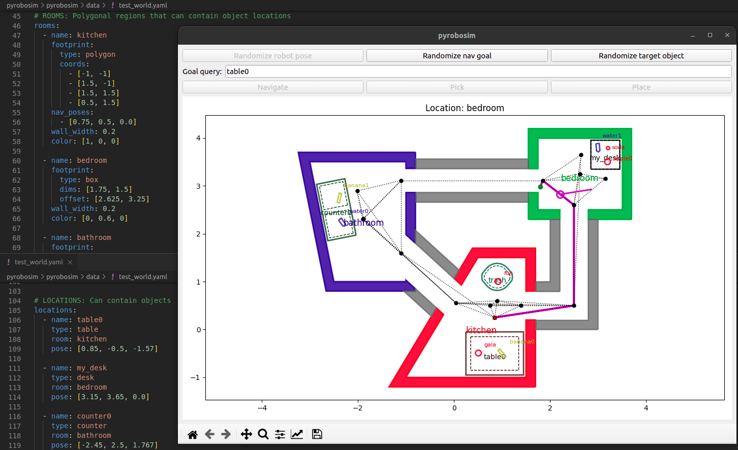
pyrobosim GUI with snippets of the world YAML file behind it.

2. Generalizing motion planning

In the original tool, navigation was as simple as possible as I was focused on real robot experiments. All I needed in the simulated world was a representative cost function for planning that would approximate how far a robot would have to travel from point A to point B.

This resulted in building up a roadmap of (known and manually specified) navigation poses around locations and at the center of rooms and hallways. Once you have this graph representation of the world, you can use a standard shortest-path search algorithm like A* to find a path between any two points in space.

This time around, I wanted a little more generality. The design has now evolved to include two popular categories of motion planners.

  • Single-query planners: Plans once from the current state of the robot to a specific goal pose. An example is the ubiquitous Rapidly-expanding Random Tree (RRT). Since each robot plans from its current state, single-query planners are considered to be properties of an individual robot in pyrobosim.
  • Multi-query planners: Builds a representation for planning which can be reused for different start/goal configurations given the world does not change. The original hard-coded roadmap fits this bill, as well as the sampling-based Probabilistic Roadmap (PRM). Since multiple robots could reuse these planners by connecting start and goal poses to an existing graph, multi-query planners are considered properties of the world itself in pyrobosim.

I also wanted to consider path following algorithms in the future. For now, the piping is there for robots to swap out different path followers, but the only implementation is a “straight line executor”. This assumes the robot is a point that can move in ideal straight-line trajectories. Later on, I would like to consider nonholonomic constraints and enable dynamically feasible planning, as well as true path following which sets the velocity of the robot within some limits rather than teleporting the robot to ideally follow a given path.

In general, there are lots of opportunities to add more of the low-level robot dynamics to pyrobosim, whereas right now the focus is largely on the higher-level behavior side. Something like the MATLAB based Mobile Robotics Simulation Toolbox, which I worked on in a former job, has more of this in place, so it’s certainly possible!

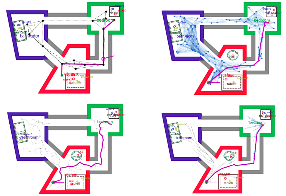
Sample path planners in pyrobosim.
Hard-coded roadmap (upper left), Probabilistic Roadmap (PRM) (upper right).
Rapidly-expanding Random Tree (RRT) (lower left), Bidirectional RRT* (lower right).

3. Plugging into the latest ecosystem

This was probably the most selfish and unnecessary update to the tools. I wanted to play with ROS2, so I made this into a ROS2 package. Simple as that. However, I throttled back on the selfishness enough to ensure that everything could also be run standalone. In other words, I don’t want to require anyone to use ROS if they don’t want to.

The ROS approach does provide a few benefits, though:

  • Distributed execution: Running the world model, GUI, motion planners, etc. in one process is not great, and in fact I ran into a lot of snags with multithreading before I introduced ROS into the mix and could split pieces into separate nodes.
  • Multi-language interaction: ROS in general is nice because you can have for example Python nodes interacting with C++ nodes “for free”. I am especially excited for this to lead to collaborations with interesting robotics tools out in the wild.

The other thing that came with this was the Gazebo world exporting, which was already available in the former code. However, there is now a newer Ignition Gazebo and I wanted to try that as well. After discovering that polyline geometries (a key feature I relied on) was not supported in Ignition, I complained just loudly enough on Twitter that the lead developer of Gazebo personally let me know when she merged that PR! I was so excited that I installed the latest version of Ignition from source shortly after and with a few tweaks to the model generation we now support both Gazebo classic and Ignition.

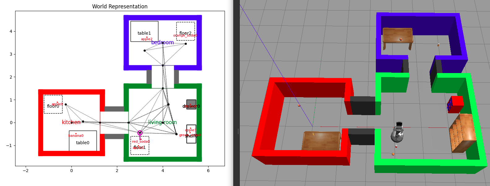
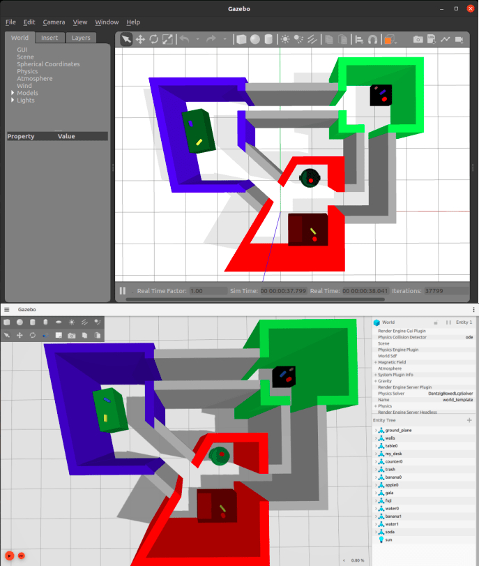
pyrobosim test world exported to Gazebo classic (top) and Ignition Gazebo (bottom).

4. Software quality

Some other things I’ve been wanting to try for a while relate to good software development practices. I’m happy that in bringing up pyrobosim, I’ve so far been able to set up a basic Continuous Integration / Continuous Development (CI/CD) pipeline and official documentation!

For CI/CD, I decided to try out GitHub Actions because they are tightly integrated with GitHub — and critically, compute is free for public repositories! I had past experience setting up Jenkins (see my previous post), and I have to say that GitHub Actions was much easier for this “hobbyist” workflow since I didn’t have to figure out where and how to host the CI server itself.

Documentation was another thing I was deliberate about in this redesign. I was always impressed when I went into some open-source package and found professional-looking documentation with examples, tutorials, and a full API reference. So I looked around and converged on Sphinx which generates the HTML documentation, and comes with an autodoc module that can automatically convert Python docstrings to an API reference. I then used ReadTheDocs which hosts the documentation online (again, for free) and automatically rebuilds it when you push to your GitHub repository. The final outcome was this pyrobosim documentation page.

The result is very satisfying, though I must admit that my unit tests are… lacking at the moment. However, it should be super easy to add new tests into the existing CI/CD pipeline now that all the infrastructure is in place! And so, the technical debt continues building up.

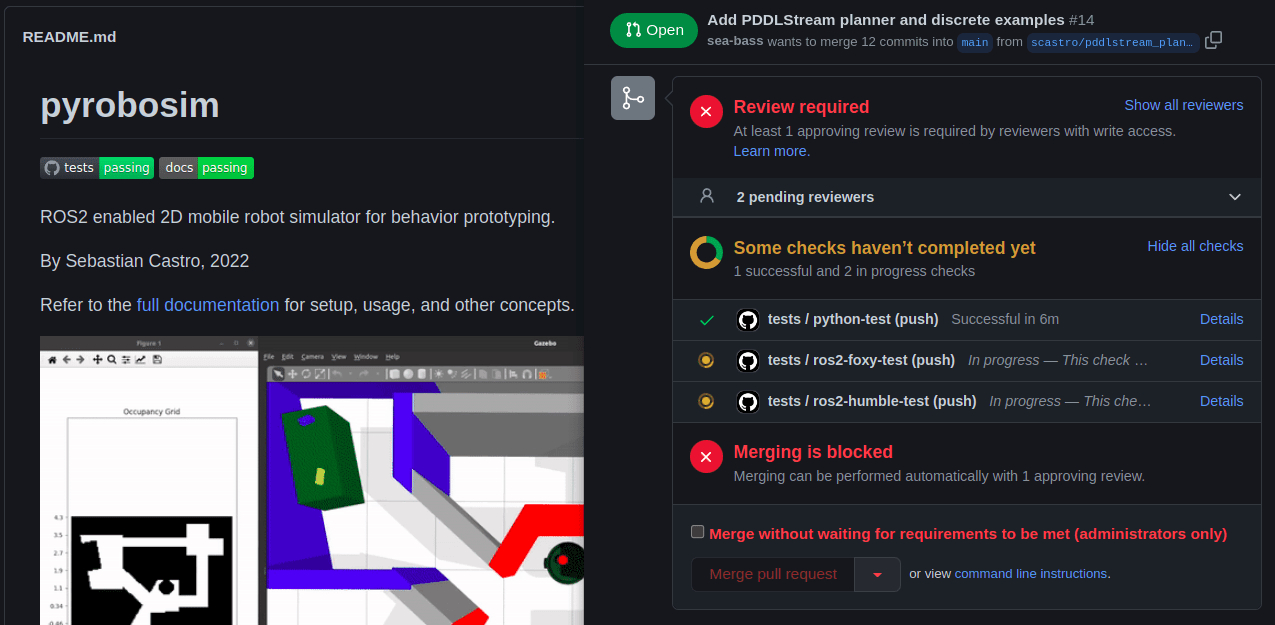
pyrobosim GitHub repo with pretty status badges (left) and automated checks in a pull request (right).

Conclusion / Next steps

This has been an introduction to pyrobosim — both its design philosophy, and the key feature sets I worked on to take the code out of its original form and into a standalone package (hopefully?) worthy of public usage. For more information, take a look at the GitHub repository and the official documentation.

Here is my short list of future ideas, which is in no way complete:

  1. Improving the existing tools: Adding more unit tests, examples, documentation, and generally anything that makes the pyrobosim a better experience for developers and users alike.
  2. Building up the navigation stack: I am particularly interested in dynamically feasible planners for nonholonomic vehicles. There are lots of great tools out there to pull from, such as Peter Corke’s Robotics Toolbox for Python and Atsushi Sakai’s PythonRobotics.
  3. Adding a behavior layer: Right now, a plan consists of a simple sequence of actions. It’s not very reactive or modular. This is where abstractions such as finite-state machines and behavior trees would be great to bring in.
  4. Expanding to multi-agent and/or partially-observable systems: Two interesting directions that would require major feature development.
  5. Collaborating with the community!

It would be fantastic to work with some of you on pyrobosim. Whether you have feedback on the design itself, specific bug reports, or the ability to develop new examples or features, I would appreciate any form of input. If you end up using pyrobosim for your work, I would be thrilled to add your project to the list of usage examples!

Finally: I am currently in the process of setting up task and motion planning with pyrobosim. Stay tuned for that follow-on post, which will have lots of cool examples.

Introduction to behavior trees

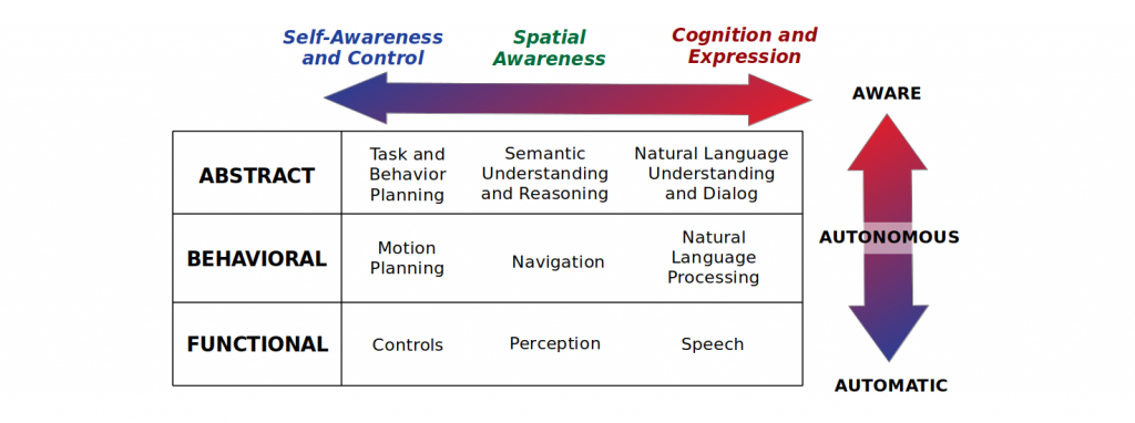
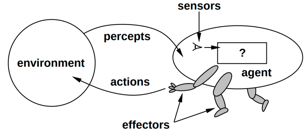
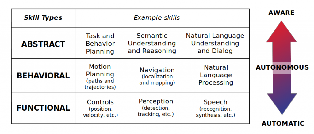
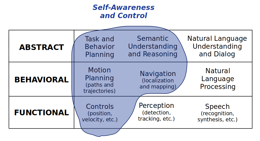
Abstraction in programming has evolved our use of computers from basic arithmetic operations to representing complex real-world phenomena using models. More specific to robotics, abstraction has moved us from low-level actuator control and basic sensing to reasoning about higher-level concepts behaviors, as I define in my Anatomy of a Robotic System post.

In autonomous systems, we have seen an entire host of abstractions beyond “plain” programming for behavior modeling and execution. Some common ones you may find in the literature include teleo-reactive programs, Petri nets, finite-state machines (FSMs), and behavior trees (BTs). In my experience, FSMs and BTs are the two abstractions you see most often today.

In this post, I will introduce behavior trees with all their terminology, contrast them with finite-state machines, share some examples and software libraries, and as always leave you with some resources if you want to learn more.

What is a behavior tree?

As we introduced above, there are several abstractions to help design complex behaviors for an autonomous agent. Generally, these consist of a finite set of entities that map to particular behaviors or operating modes within our system, e.g., “move forward”, “close gripper”, “blink the warning lights”, “go to the charging station”. Each model class has some set of rules that describe when an agent should execute each of these behaviors, and more importantly how the agent should switch between them.

Behavior trees (BTs) are one such abstraction, which I will define by the following characteristics:

  1. Behavior trees are trees (duh): They start at a root node and are designed to be traversed in a specific order until a terminal state is reached (success or failure).
  2. Leaf nodes are executable behaviors: Each leaf will do something, whether it’s a simple check or a complex action, and will output a status (success, failure, or running). In other words, leaf nodes are where you connect a BT to the lower-level code for your specific application.
  3. Internal nodes control tree traversal: The internal (non-leaf) nodes of the tree will accept the resulting status of their children and apply their own rules to dictate which node should be expanded next.

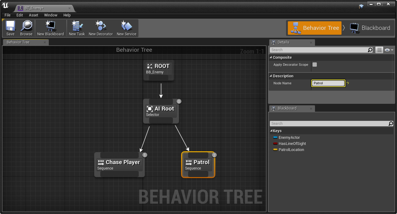
Behavior trees actually began in the videogame industry to define behaviors for non-player characters (NPCs): Both Unreal Engine and Unity (two major forces in this space) have dedicated tools for authoring BTs. This is no surprise; a big advantage of BTs is that they are easy to compose and modify, even at runtime. However, this sacrifices the ease of designing reactive behaviors (for example, mode switches) compared to some of the other abstractions, as you will see later in this post.

Since then, BTs have also made it into the robotics domain as robots have become increasingly capable of doing more than simple repetitive tasks. Easily the best resource here is the textbook “Behavior Trees in Robotics and AI: An Introduction” by Michele Colledanchise and Petter Ögren. In fact, if you really want to learn the material you should stop reading this post and go directly to the book … but please stick around?

Behavior tree Editor in Unreal Engine. Source: Unreal Engine documentation

Behavior tree terminology

Let’s dig into the terminology in behavior trees. While the language is not standard across the literature and various software libraries, I will largely follow the definitions in Behavior Trees in Robotics and AI.

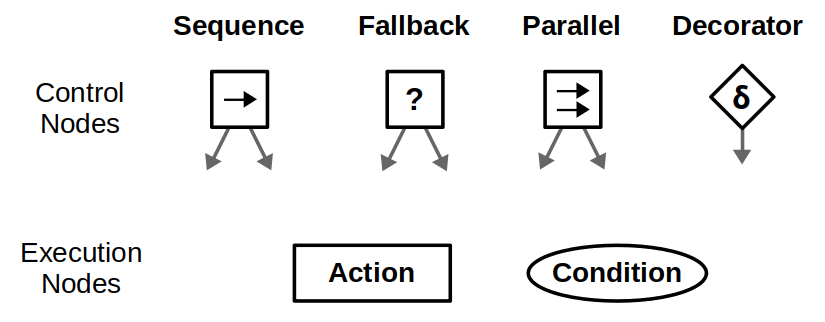
At a glance, these are the types of nodes that make up behavior trees and how they are represented graphically:

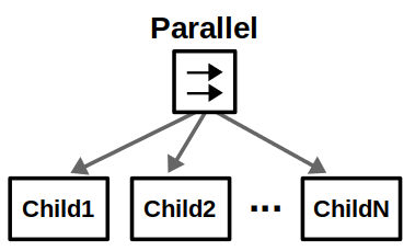
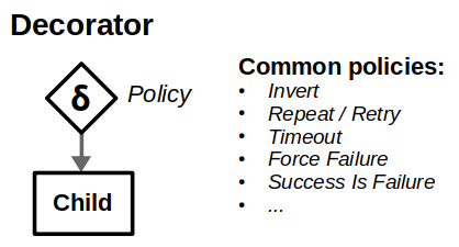
Overview of behavior tree nodes.

Behavior trees execute in discrete update steps known as ticks. When a BT is ticked, usually at some specified rate, its child nodes recursively tick based on how the tree is constructed. After a node ticks, it returns a status to its parent, which can be Success, Failure, or Running.

Execution nodes, which are leaves of the BT, can either be Action or Condition nodes. The only difference is that condition nodes can only return Success or Failure within a single tick, whereas action nodes can span multiple ticks and can return Running until they reach a terminal state. Generally, condition nodes represent simple checks (e.g., “is the gripper open?”) while action nodes represent complex actions (e.g., “open the door”).

Control nodes are internal nodes and define how to traverse the BT given the status of their children. Importantly, children of control nodes can be execution nodes or control nodes themselves. Sequence, Fallback, and Parallel nodes can have any number of children, but differ in how they process said children. Decorator nodes necessarily have one child, and modify its behavior with some custom defined policy.

Check out the images below to see how the different control nodes work.

Sequence nodes execute children in order until one child returns Failure or all children returns Success.
Fallback nodes execute children in order until one of them returns Success or all children return Failure. These nodes are key in designing recovery behaviors for your autonomous agents.
Parallel nodes will execute all their children in “parallel”. This is in quotes because it’s not true parallelism; at each tick, each child node will individually tick in order. Parallel nodes return Success when at least M child nodes (between 1 and N) have succeeded, and Failure when all child nodes have failed.
Decorator nodes modify a single child node with a custom policy. A decorator has its own set of rules for changing the status of the “decorated node”. For example, an “Invert” decorator will change Success to Failure, and vice-versa. While decorators can add flexibility to your behavior tree arsenal, you should stick to standard control nodes and common decorators as much as possible so others can easily understand your design.

Robot example: searching for objects

The best way to understand all the terms and graphics in the previous section is through an example. Suppose we have a mobile robot that must search for specific objects in a home environment. Assume the robot knows all the search locations beforehand; in other words, it already has a world model to operate in.

Our mobile robot example. A simulated TurtleBot3 must move in a known map to find blocks of a given color.

Let’s start simple. If there is only one location (we’ll call it A), then the BT is a simple sequence of the necessary actions: Go to the location and then look for the object.

Our first behavior tree. Bask in the simplicity while you can…

We’ve chosen to represent navigation as an action node, as it may take some time for the robot to move (returning Running in the process). On the other hand, we represent vision as a condition node, assuming the robot can detect the object from a single image once it arrives at its destination. I admit, this is totally contrived for the purpose of showing one of each execution node.

One very common design principle you should know is defined in the book as explicit success conditions. In simpler terms, you should almost always check before you act. For example, if you’re already at a specific location, why not check if you’re already there before starting a navigation action?

Explicit success conditions use a Fallback node with a condition preceding an action. The guarded action will only execute if the success condition is not met — in this example if the robot is not at location A

Our robot likely operates in an environment with multiple locations, and the idea is to look in all possible locations until we find the object of interest. This can be done by introducing a root-level Fallback node and repeating the above behavior for each location in some specified order.

We can also use Fallback nodes to define reactive behaviors; that is, if one behavior does not work, try the next one, and so on.

Finally, suppose that instead of looking for a single object, we want to consider several objects — let’s say apples and oranges. This use case of composing conditions can be done with Parallel nodes as shown below.

  • If we accept either an apple or an orange (“OR” condition), then we succeed if one node returns Success.
  • If we require both an apple and an orange (“AND” condition), then we succeed if both nodes return Success.
  • If we care about the order of objects, e.g., you must find an apple before finding an orange, then this could be done with a Sequence node instead.
Parallel nodes allows multiple actions and/or conditions to be considered within a single tick.

Of course, you can also compose actions in parallel — for example, turning in place until a person is detected for 5 consecutive ticks. While my example is hopefully simple enough to get the basics across, I highly recommend looking at the literature for more complex examples that really show off the power of BTs.

Robot example revisited: decorators and blackboards

I don’t know about you, but looking at the BT above leaves me somewhat uneasy. It’s just the same behavior copied and pasted multiple times underneath a Fallback node. What if you had 20 different locations, and the behavior at each location involved more than just two simplified execution nodes? Things could quickly get messy.

In most software libraries geared for BTs you can define these execution nodes as parametric behaviors that share resources (for example, the same ROS action client for navigation, or object detector for vision). Similarly, you can write code to build complex trees automatically and compose them from a ready-made library of subtrees. So the issue isn’t so much efficiency, but readability.

There is an alternative implementation for this BT, which can extend to many other applications. Here’s the basic idea:

  • Introduce decorators: Instead of duplicating the same subtree for each location, have a single subtree and decorate it with a policy that repeats the behavior until successful.
  • Update the target location at each iteration: Suppose you now have a “queue” of target locations to visit, so at each iteration of the subtree you pop an element from that queue. If the queue eventually ends up empty, then our BT fails.

In most BTs, we often need some notion of shared data like the location queue we’re discussing. This is where the concept of a blackboard comes in: you’ll find blackboard constructs in most BT libraries out there, and all they really are is a common storage area where individual behaviors can read or write data.

Our example BT could now be refactored as follows. We introduce a “GetLoc” action that pops a location from our queue of known locations and writes it to the blackboard as some parameter target_location. If the queue is empty, this returns Failure; otherwise it returns Success. Then, downstream nodes that deal with navigation can use this target_location parameter, which changes every time the subtree repeats.

The addition of a blackboard and a “Repeat” decorator can greatly simplify our tree even if the underlying behavior is the same.

You can use blackboards for many other tasks. Here’s another extension of our example: Suppose that after finding an object, the robot should speak with the object it detected, if any. So, the “FoundApple” and “FoundOrange” conditions could write to a located_objects parameter in the blackboard and a subsequent “Speak” action would read it accordingly. A similar solution could be applied, for instance, if the robot needs to pick up the detected object and has different manipulation policies depending on the type of object.

Fun fact: This section actually came from a real discussion with Davide Faconti, in which… he essentially schooled me. It brings me great joy to turn my humiliation into an educational experience for you all.

Behavior tree software libraries

Let’s talk about how to program behavior trees! There are quite a few libraries dedicated to BTs, but my two highlights in the robotics space are py_trees and BehaviorTree.CPP.

py_trees is a Python library created by Daniel Stonier.

  • Because it uses an interpreted language like Python, the interface is very flexible and you can basically do what you want… which has its pros and cons. I personally think this is a good choice if you plan on automatically modifying behavior trees at run time.
  • It is being actively developed and with every release you will find new features. However, many of the new developments — not just additional decorators and policy options, but the visualization and logging tools — are already full-steam-ahead with ROS 2. So if you’re still using ROS 1 you will find yourself missing a lot of new things. Check out the PyTrees-ROS Ecosystem page for more details.
  • Some of the terminology and design paradigms are a little bit different from the Behavior Trees in Robotics book. For example, instead of Fallback nodes this library uses Selector nodes, and these behave slightly differently.
Our navigation example using the py_trees library and rqt_py_trees for visualization.

BehaviorTree.CPP is a C++ library developed by Davide Faconti and Michele Colledanchise (yes, one of the book authors). It should therefore be no surprise that this library follows the book notation much more faithfully.

  • This library is quickly gaining traction as the behavior tree library of the ROS developers’ ecosystem, because C++ is similarly the language of production quality development for robotics. In fact, the official ROS 2 navigation stack uses this library in its BT Navigator feature.
  • It heavily relies on an XML based workflow, meaning that the recommended way to author a BT is through XML files. In your code, you register node types with user-defined classes (which can inherit from a rich library of existing classes), and your BT is automatically synthesized!
  • It is paired with a great tool named Groot which is not only a visualizer, but a graphical interface for editing behavior trees. The XML design principle basically means that you can draw a BT and export it as an XML file that plugs into your code.
  • This all works wonderfully if you know the structure of your BT beforehand, but leaves a little to be desired if you plan to modify your trees at runtime. Granted, you can also achieve this using the programmatic approach rather than XML, but this workflow is not documented/recommended, and doesn’t yet play well with the visualization tools.
Our navigation example using the BehaviorTree.CPP library and Groot for visualization.

So how should you choose between these two libraries? They’re both mature, contain a rich set of tools, and integrate well with the ROS ecosystem. It ultimately boils down to whether you want to use C++ or Python for your development. In my example GitHub repo I tried them both out, so you can decide for yourself!

Behavior trees vs. finite-state machines

In my time at MathWorks, I was immersed in designing state machines for robotic behavior using Stateflow — in fact, I even did a YouTube livestream on this topic. However, robotics folks often asked me if there were similar tools for modeling behavior trees, which I had never heard of at the time. Fast forward to my first day at CSAIL, my colleague at the time (Daehyung Park) showed me one of his repositories and I finally saw my first behavior tree. It wasn’t long until I was working with them in my project as a layer between planning and execution, which I describe in my 2020 recap blog post.

As someone who has given a lot of thought to “how is a BT different from a FSM?”, I wanted to reaffirm that they both have their strengths and weaknesses, and the best thing you can do is learn when a problem is better suited for one or the other (or both).

The Behavior Trees in Robotics and AI book expands on these thoughts in way more rigor, but here is my attempt to summarize the key ideas:

  • In theory, it is possible to express anything as a BT, FSM, one of the other abstractions, or as plain code. However, each model has its own advantages and disadvantages in their intent to aid design at larger scale.
  • Specific to BTs vs. FSMs, there is a tradeoff between modularity and reactivity. Generally, BTs are easier to compose and modify while FSMs have their strength in designing reactive behaviors.

Let’s use another robotics example to go deeper into these comparisons. Suppose we have a picking task where a robot must move to an object, grab it by closing its gripper, and then move back to its home position. A side-by-side BT and FSM comparison can be found below. For a simple design like this, both implementations are relatively clean and easy to follow.

Behavior tree (left) and finite-state machine (right) for our robot picking example.

Now, what happens if we want to modify this behavior? Say we first want to check whether the pre-grasp position is valid, and correct if necessary before closing the gripper. With a BT, we can directly insert a subtree along our desired sequence of actions, whereas with a FSM we must rewire multiple transitions. This is what we mean when we claim BTs are great for modularity.

Modifications to our BT (left) and FSM (right) if we want to add a pre-grasp correction behavior.

On the other hand, there is the issue of reactivity. Suppose our robot is running on a finite power source, so if the battery is low it must return to the charging station before returning to its task. You can implement something like this with BTs, but a fully reactive behavior (that is, the battery state causes the robot to go charge no matter where it is) is easier to implement with a FSM… even if it looks a bit messy.

On the note of “messy”, behavior tree zealots tend to make the argument of “spaghetti state machines” as reasons why you should never use FSMs. I believe that is not a fair comparison. The notion of a hierarchical finite-state machine (HFSM) has been around for a long time and helps avoid this issue if you follow good design practices, as you can see below. However, it is true that managing transitions in a HFSM is still more difficult than adding or removing subtrees in a BT.

There have been specific constructs defined to make BTs more reactive for exactly these applications. For example, there is the notion of a “Reactive Sequence” that can still tick previous children in a sequence even after they have returned Success. In our example, this would allow us to terminate a subtree with Failure if the battery levels are low at any point during that action sequence, which may be what we want.

Adding a battery check and charging action to a BT is easy, but note that this check is not reactive — it only occurs at the start of the sequence. Implementing more reactivity would complicate the design of the BT, but is doable with constructs like Reactive Sequences.
FSMs can allow this reactivity by allowing the definition of transitions between any two states.
Hierarchical FSMs can clean up the diagram. In this case, we define a superstate named “Nominal”, thus defining two clear operating modes between normal operation and charging.

Because of this modularity / reactivity tradeoff, I like to think that FSMs are good at managing higher-level operating modes (such as normal operation vs. charging), and BTs are good at building complex sequences of behaviors that are excellent at handling recoveries from failure. So, if this design were up to me, it might be a hybrid that looks something like this:

Best of both worlds: High-level mode switches are handled by a FSM and mode-specific behaviors are managed with BTs.

Conclusion

Thank for reading through this introductory post, and I look forward to your comments, questions, and suggestions. If you want to try the code examples, check out my example GitHub repository.

To learn more about behavior trees, here are some good resources that I’ve relied on over the past year and a bit.

See you next time!

Anatomy of a robotic system

Robotics is both an exciting and intimidating field because it takes so many different capabilities and disciplines to spin up a robot. This goes all the way from mechatronic design and hardware engineering to some of the more philosophical parts of software engineering.

Those who know me also know I’m a total “high-level guy”. I’m fascinated by how complex a modern robotic system is and how all the pieces come together to make something that’s truly impressive. I don’t have particularly deep knowledge in any specific area of robotics, but I appreciate the work of countless brilliant people that give folks like me the ability to piece things together.

In this post, I will go through what it takes to put together a robot that is highly capable by today’s standards. This is very much an opinion article that tries to slice robotic skills along various dimensions. I found it challenging to find a single “correct” taxonomy, so I look forward to hearing from you about anything you might disagree with or have done differently.

What defines a robot?

Roughly speaking, a robot is a machine with sensors, actuators, and some computing device that has been programmed to perform some level of autonomous behavior. Below is the essential “getting started” diagram that anyone in AI should recognize.

Diagram of typical artificially intelligent agent, such as a robot. Source: Artificial Intelligence: A Modern Approach (Russell, Norvig)

This opens up the ever present “robot vs. machine” debate that I don’t want to spent too much time on, but my personal distinction between a robot vs. a machine includes a couple of specifications.

  1. A robot has at least one closed feedback loop between sensing and actuation that does not require human input. This discounts things like a remote-controlled car, or a machine that constantly executes a repetitive motion but will never recover if you nudge it slightly — think, for example, Theo Jansen’s kinetic sculptures.
  2. A robot is an embodied agent that operates in the physical world. This discounts things like chatbots, or even smart speakers which — while awesome displays of artificial intelligence — I wouldn’t consider them to be robots… yet.

The big picture: Automatic, Autonomous, and Aware

Robots are not created equal. Not to say that simpler robots don’t have their purpose — knowing how simple or complex (technology- and budget-wise) to build a robot given the problem at hand is a true engineering challenge. To say it a different way: overengineering is not always necessary.

I will now categorize the capabilities of a robot into three bins: Automatic, Autonomous, and Aware. This roughly corresponds to how low- or high-level a robot’s skills have been developed, but it’s not an exact mapping as you will see.

Don’t worry too much about the details in the table as we will cover them throughout the post.

Automatic: The robot is controllable and it can execute motion commands provided by a human in a constrained environment. Think, for example, of industrial robots in an assembly line. You don’t need to program very complicated intelligence for a robot to put together a piece of an airplane from a fixed set of instructions. What you need is fast, reliable, and sustained operation. The motion trajectories of these robots are often trained and calibrated by a technician for a very specific task, and the surroundings are tailored for robots and humans to work with minimal or no conflict.

Autonomous: The robot can now execute tasks in an uncertain environment with minimal human supervision. One of the most pervasive example of this is self-driving cars (which I absolutely label as robots). Today’s autonomous vehicles can detect and avoid other cars and pedestrians, perform lane-change maneuvers, and navigate the rules of traffic with fairly high success rates despite the negative media coverage they may get for not being 100% perfect.

Aware: This gets a little bit into the “sci-fi” camp of robots, but rest assured that research is bringing this closer to reality day by day. You could tag a robot as aware when it can establish two-way communication with humans. An aware robot, unlike the previous two categories, is not only a tool that receives commands and makes mundane tasks easier, but one that is perhaps more collaborative. In theory, aware robots can understand the world at a higher level of abstraction than their more primitive counterparts, and process humans’ intentions from verbal or nonverbal cues, still under the general goal of solving a real-life problem.

A good example is a robot that can help humans assemble furniture. It operates in the same physical and task space as us humans, so it should adapt to where we choose to position ourselves or what part of the furniture we are working on without getting in the way. It can listen to our commands or requests, learn from our demonstrations, and tell us what it sees or what it might do next in language we understand so we can also take an active part in ensuring the robot is being used effectively.

Self-awareness and control: How much does the robot know about itself?
Spatial awareness: How much does the robot know about the environment and its own relationship to the environment?
Cognition and expression: How capable is the robot about reasoning about the state of the world and expressing its beliefs and intentions to humans or other autonomous agents?

Above you can see a perpendicular axis of categorizing robot awareness. Each highlighted area represents the subset of skills it may require for a robot to achieve awareness on that particular dimension. Notice how forming abstractions — i.e., semantic understanding and reasoning — is crucial for all forms of awareness. That is no coincidence.

The most important takeaway as we move from automatic to aware is the increasing ability for robots to operate “in the wild”. Whereas an industrial robot may be designed to perform repetitive tasks with superhuman speed and strength, a home service robot will often sacrifice this kind of task-specific performance with more generalized skills needed for human interaction and navigating uncertain and/or unknown environments.

A Deeper Dive Into Robot Skills

Spinning up a robot requires a combination of skills at different levels of abstraction. These skills are all important aspects of a robot’s software stack and require vastly different areas of expertise. This goes back to the central point of this blog post: it’s not easy to build a highly capable robot, and it’s certainly not easy to do it alone!

Functional Skills

This denotes the low-level foundational skills of a robot. Without a robust set of functional skills, you would have a hard time getting your robot to be successful at anything else higher up the skill chain.

Being at the lowest level of abstraction, functional skills are closely tied to direct interaction with the actuators and sensor of the robot. Indeed, these skills can be discussed along the acting and sensing modalities.

Acting

  • Controls is all about ensuring the robot can reliably execute physical commands — whether this is a wheeled robot, flying robot, manipulator, legged robot, soft robot (… you get the point …) it needs to respond to inputs in a predictable way if it is to interact with the world. It’s a simple concept, but a challenging task that ranges from controlling electrical current/fluid pressure/etc. to multi-actuator coordination towards executing a full motion trajectory.
  • Speech synthesis acts on the physical world in a different way — this is more on the human-robot interaction (HRI) side of things. You can think of these capabilities as the robot’s ability to express its state, beliefs, and intentions in a way that is interpretable by humans. Imagine speech synthesis as more than speaking in a monotone robotic voice, but maybe simulating emotion or emphasis to help get information across to the human. This is not limited to speech. Many social robots will also employ visual cues like facial expressions, lights and colors, or movements — for example, look at MIT’s Leonardo.

Sensing

  • Controls requires some level of proprioceptive (self) sensing. To regulate the state of a robot, we need to employ sensors like encoders, inertial measurement units, and so on.
  • Perception, on the other hand, deals with exteroceptive (environmental) sensing. This mainly deals with line-of-sight sensors like sonar, radar, and lidar, as well as cameras. Perception algorithms require significant processing to make sense of a bunch of noisy pixels and/or distance/range readings. The act of abstracting this data to recognize and locate objects, track them over space and time, and use them for higher-level planning is what makes it exciting and challenging. Finally, back on the social robotics topic, vision can also enable robots to infer the state of humans for nonverbal communication.
  • Speech recognition is another form of exteroceptive sensing. Getting from raw audio to accurate enough text that the robot can process is not trivial, despite how easy smart assistants like Google Assistant, Siri, and Alexa have made it look. This field of work is officially known as automatic speech recognition (ASR).

Behavioral Skills

Behavioral skills are a step above the more “raw” sensor-to-actuator processing loops that we explored in the Functional Skills section. Creating a solid set of behavioral skills simplifies our interactions with robots both as users and programmers.

At the functional level, we have perhaps demonstrated capabilities for the robot to respond to very concrete, mathematical goals. For example,

  • Robot arm: “Move the elbow joint to 45 degrees and the shoulder joint to 90 degrees in less than 2.5 seconds with less than 10% overshoot. Then, apply a force of 2 N on the gripper.”
  • Autonomous car: “Speed up to 40 miles per hour without exceeding acceleration limit of 0.1 g and turn the steering wheel to attain a turning rate of 10 m.”

At the behavioral level, commands may take the form of:

  • Robot arm: “Grab the door handle.”
  • Autonomous car: “Turn left at the next intersection while following the rules of traffic and passenger ride comfort limits.”
  • Abstracting away these motion planning and navigation tasks requires a combination of models of the robot and/or world, and of course, our set of functional skills like perception and control.

  • Motion planning seeks to coordinate multiple actuators in a robot to execute higher-level tasks. Instead of moving individual joints to setpoints, we now employ kinematic and dynamic models of our robot to operate in the task space — for example, the pose of a manipulator’s end effector or the traffic lane a car occupies in a large highway. Additionally, to go from a start to a goal configuration requires path planning and a trajectory that dictates how to execute the planned path over time. I like this set of slides as a quick intro to motion planning.
  • Navigation seeks to build a representation of the environment (mapping) and knowledge of the robot’s state within the environment (localization) to enable the robot to operate in the world. This representation could be in the form of simple primitives like polygonal walls and obstacles, an occupancy grid, a high-definition map of highways, etc.

If this hasn’t yet got across, behavioral skills and functional skills definitely do not work in isolation. Motion planning in a space with obstacles requires perception and navigation. Navigating in a world requires controls and motion planning.

On the language side, Natural Language Processing (NLP) is what takes us from raw text input — whether it came from speech or directly typed in — to something more actionable for the robot. For instance, if a robot is given the command “bring me a snack from the kitchen”, the NLP engine needs to interpret this at the appropriate level to perform the task. Putting it all together,

  1. Going to the kitchen is a navigation problem that likely requires a map of the house.
  2. Locating the snack and getting its 3D position relative to the robot is a perception problem.
  3. Picking up the snack without knocking other things over is a motion planning problem.
  4. Returning to wherever the human was when the command was issued is again a navigation problem. Perhaps someone closed a door along the way, or left something in the way, so the robot may have to replan based on these changes to the environment.

Abstract Skills

Simply put, abstract skills are the bridge between humans and robot behaviors. All the skills in the row above perform some transformation that lets humans more easily express their commands to robots, and similarly lets robots more easily express themselves to humans.

Task and Behavior Planning operates on the key principles of abstraction and composition. A command like “get me a snack from the kitchen” can be broken down into a set of fundamental behaviors (navigation, motion planning, perception, etc.) that can be parameterized and thus generalized to other types of commands such as “put the bottle of water in the garbage”. Having a common language like this makes it useful for programmers to add capabilities to robots, and for users to leverage their robot companions to solve a wider set of problems. Modeling tools such as finite-state machines and behavior trees have been integral in implementing such modular systems.

Semantic Understanding and Reasoning is bringing abstract knowledge to a robot’s internal model of the world. For example, in navigation we saw that a map can be represented as “occupied vs. unoccupied”. In reality, there are more semantics that can enrich the task space of the robot besides “move here, avoid there”. Does the environment have separate rooms? Is some of the “occupied space” movable if needed? Are there elements in the world where objects can be stored and retrieved? Where are certain objects typically found such that the robot can perform a more targeted search? This recent paper from Luca Carlone’s group is a neat exploration into maps with rich semantic information, and a huge portal of future work that could build on this.

Natural Language Understanding and Dialog is effectively two-way communication of semantic understanding between humans and robots. After all, the point of abstracting away our world model was so we humans could work with it more easily. Here are examples of both directions of communication:

  • Robot-to-human: If a robot failed to execute a plan or understand a command, can it actually tell the human why it failed? Maybe a door was locked on the way to the goal, or the robot did not know what a certain word meant and it can ask you to define it.
  • Human-to-robot: The goal here is to share knowledge with the robot to enrich its semantic understanding the world. Some examples might be teaching new skills (“if you ever see a mug, grab it by the handle”) or reducing uncertainty about the world (“the last time I saw my mug it was on the coffee table”).

This is all a bit of a pipe dream — Can a robot really be programmed to work with humans at such a high level of interaction? It’s not easy, but research tries to tackle problems like these every day. I believe a good measure of effective human-robot interaction is whether the human and robot jointly learn not to run into the same problem over and over, thus improving the user experience.

Conclusion

Thanks for reading, even if you just skimmed through the pictures. I hope this was a useful guide to navigating robotic systems that was somewhat worth its length. As I mentioned earlier, no categorization is perfect and I invite you to share your thoughts.

Going back to one of my specifications: A robot has at least one closed feedback loop between sensing and actuation that does not require human input. Let’s try put our taxonomy in an example set of feedback loops below. Note that I’ve condensed the natural language pipeline into the “HRI” arrows connecting to the human.

Example of a hierarchical robotic system architecture. Icons made by Freepik from www.flaticon.com

Because no post today can evade machine learning, I also want to take some time make readers aware of machine learning’s massive role in modern robotics.

  • Processing vision and audio data has been an active area of research for decades, but the rise of neural networks as function approximators for machine learning (i.e. “deep learning”) has made recent perception and ASR systems more capable than ever.
  • Additionally, learning has demonstrated its use at higher levels of abstraction. Text processing with neural networks has moved the needle on natural language processing and understanding. Similarly, neural networks have enabled end-to-end systems that can learn to produce motion, task, and/or behavior plans from complex observation sources like images and range sensors.

The truth is, our human knowledge is being outperformed by machine learning for processing such high-dimensional data. Always remember that machine learning shouldn’t be a crutch due to its biggest pitfall: We can’t (yet) explain why learned systems behave the way they do, which means we can’t (yet) formulate the kinds guarantees than we can with traditional methods. The hope is to eventually refine our collective scientific knowledge so we’re not relying on data-driven black-box approaches. After all, knowing how and why robots learn will only make them more capable in the future.

On that note, you have earned yourself a break from reading. Until next time!