TL; DR
The fastest way to stall an agentic AI project is to reuse a workflow that no longer fits. Using syftr, we identified “silver bullet” flows for both low-latency and high-accuracy priorities that consistently perform well across multiple datasets. These flows outperform random seeding and transfer learning early in optimization. They recover about 75% of the performance of a full syftr run at a fraction of the cost, which makes them a fast starting point but still leaves room to improve.
If you have ever tried to reuse an agentic workflow from one project in another, you know how often it falls flat. The model’s context length might not be enough. The new use case might require deeper reasoning. Or latency requirements might have changed.
Even when the old setup works, it may be overbuilt – and overpriced – for the new problem. In those cases, a simpler, faster setup might be all you need.
We set out to answer a simple question: Are there agentic flows that perform well across many use cases, so you can choose one based on your priorities and move forward?
Our research suggests the answer is yes, and we call them “silver bullets.”
We identified silver bullets for both low-latency and high-accuracy goals. In early optimization, they consistently beat transfer learning and random seeding, while avoiding the full cost of a full syftr run.
In the sections that follow, we explain how we found them and how they stack up against other seeding strategies.
A quick primer on Pareto-frontiers
You don’t need a math degree to follow along, but understanding the Pareto-frontier will make the rest of this post much easier to follow.
Figure 1 is an illustrative scatter plot – not from our experiments – showing completed syftr optimization trials. Sub-plot A and Sub-plot B are identical, but B highlights the first three Pareto-frontiers: P1 (red), P2 (green), and P3 (blue).
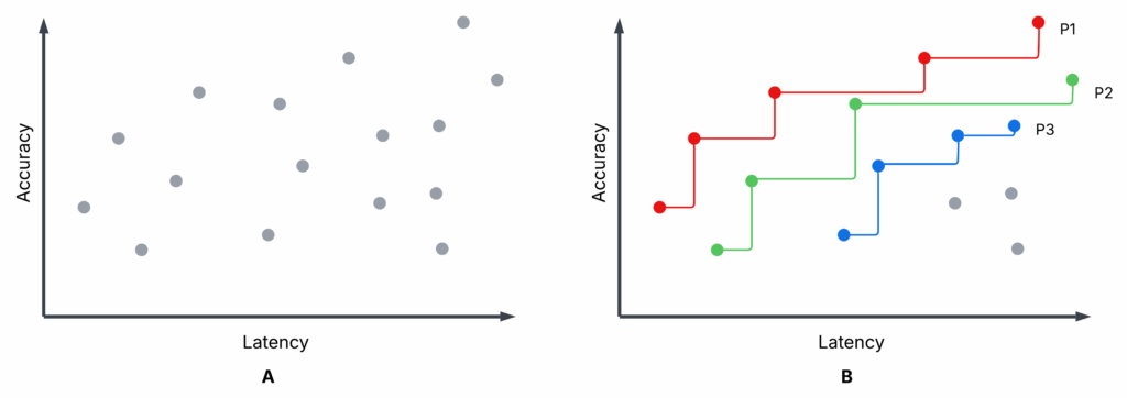
- Each trial: A specific flow configuration is evaluated on accuracy and average latency (higher accuracy, lower latency are better).
- Pareto-frontier (P1): No other flow has both higher accuracy and lower latency. These are non-dominated.
- Non-Pareto flows: At least one Pareto flow beats them on both metrics. These are dominated.
- P2, P3: If you remove P1, P2 becomes the next-best frontier, then P3, and so on.
You might choose between Pareto flows depending on your priorities (e.g., favoring low latency over maximum accuracy), but there’s no reason to choose a dominated flow — there’s always a better option on the frontier.
Optimizing agentic AI flows with syftr
Throughout our experiments, we used syftr to optimize agentic flows for accuracy and latency.
This approach allows you to:
- Select datasets containing question–answer (QA) pairs
- Define a search space for flow parameters
- Set objectives such as accuracy and cost, or in this case, accuracy and latency
In short, syftr automates the exploration of flow configurations against your chosen objectives.
Figure 2 shows the high-level syftr architecture.
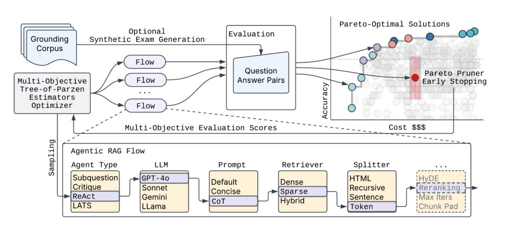
Given the practically endless number of possible agentic flow parametrizations, syftr relies on two key techniques:
- Multi-objective Bayesian optimization to navigate the search space efficiently.
- ParetoPruner to stop evaluation of likely suboptimal flows early, saving time and compute while still surfacing the most effective configurations.
Silver bullet experiments
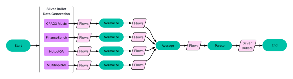
Our experiments followed a four-part process (Figure 3).
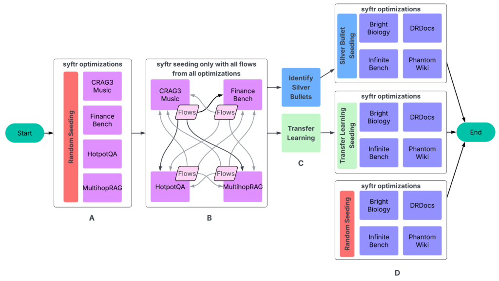
A: Run syftr using simple random sampling for seeding.
B: Run all finished flows on all other experiments. The resulting data then feeds into the next step.
C: Identifying silver bullets and conducting transfer learning.
D: Running syftr on four held-out datasets three times, using three different seeding strategies.
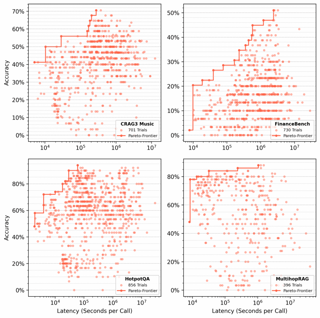
Step 1: Optimize flows per dataset
We ran several hundred trials on each of the following datasets:
- CRAG Task 3 Music
- FinanceBench
- HotpotQA
- MultihopRAG
For each dataset, syftr searched for Pareto-optimal flows, optimizing for accuracy and latency (Figure 4).
Step 3: Identify silver bullets
Once we had identical flows across all training datasets, we could pinpoint the silver bullets — the flows that are Pareto-optimal on average across all datasets.
Process:
- Normalize results per dataset. For each dataset, we normalize accuracy and latency scores by the highest values in that dataset.
- Group identical flows. We then group matching flows across datasets and calculate their average accuracy and latency.
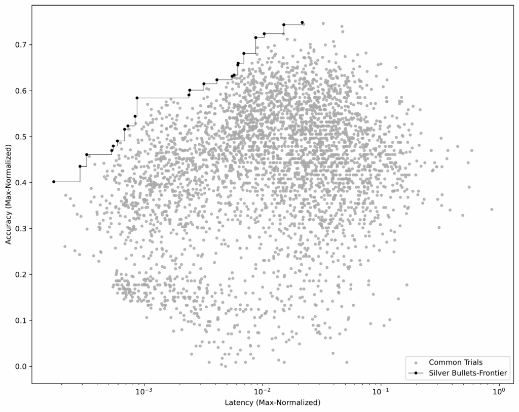
- Identify the Pareto-frontier. Using this averaged dataset (see Figure 6), we select the flows that build the Pareto-frontier.
These 23 flows are our silver bullets — the ones that perform well across all training datasets.
Step 4: Seed with transfer learning
In our original syftr paper, we explored transfer learning as a way to seed optimizations. Here, we compared it directly against silver bullet seeding.
In this context, transfer learning simply means selecting specific high-performing flows from historical (training) studies and evaluating them on held-out datasets. The data we use here is the same as for silver bullets (Figure 3).
Process:
- Select candidates. From each training dataset, we took the top-performing flows from the top two Pareto-frontiers (P1 and P2).
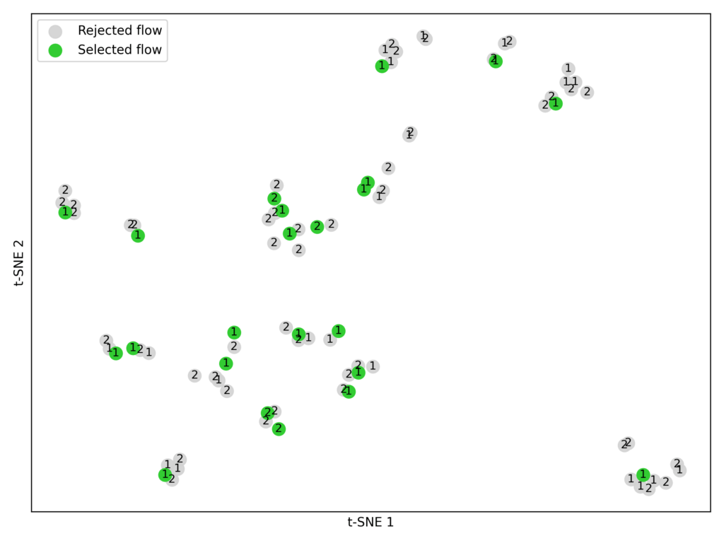
- Embed and cluster. Using the embedding model BAAI/bge-large-en-v1.5, we converted each flow’s parameters into numerical vectors. We then applied K-means clustering (K = 23) to group similar flows (Figure 7).
- Match experiment constraints. We limited each seeding strategy (silver bullets, transfer learning, random sampling) to 23 flows for a fair comparison, since that’s how many silver bullets we identified.
Note: Transfer learning for seeding isn’t yet fully optimized. We could use more Pareto-frontiers, select more flows, or try different embedding models.
Step 5: Testing it all
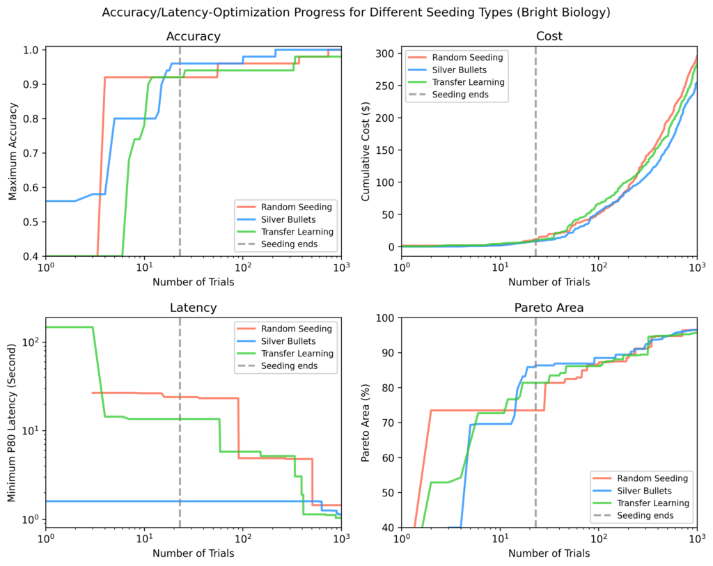
In the final evaluation phase (Step D in Figure 3), we ran ~1,000 optimization trials on four test datasets — Bright Biology, DRDocs, InfiniteBench, and PhantomWiki — repeating the process three times for each of the following seeding strategies:
- Silver bullet seeding
- Transfer learning seeding
- Random sampling
For each trial, GPT-4o-mini served as the judge, verifying an agent’s response against the ground-truth answer.
Results
We set out to answer:
Which seeding approach — random sampling, transfer learning, or silver bullets — delivers the best performance for a new dataset in the fewest trials?
For each of the four held-out test datasets (Bright Biology, DRDocs, InfiniteBench, and PhantomWiki), we plotted:
- Accuracy
- Latency
- Cost
- Pareto-area: a measure of how close results are to the optimal result
In each plot, the vertical dotted line marks the point when all seeding trials have completed. After seeding, silver bullets showed on average:
- 9% higher maximum accuracy
- 84% lower minimum latency
- 28% larger Pareto-area
compared to the other strategies.
Bright Biology
Silver bullets had the highest accuracy, lowest latency, and largest Pareto-area after seeding. Some random seeding trials did not finish. Pareto-areas for all methods increased over time but narrowed as optimization progressed.
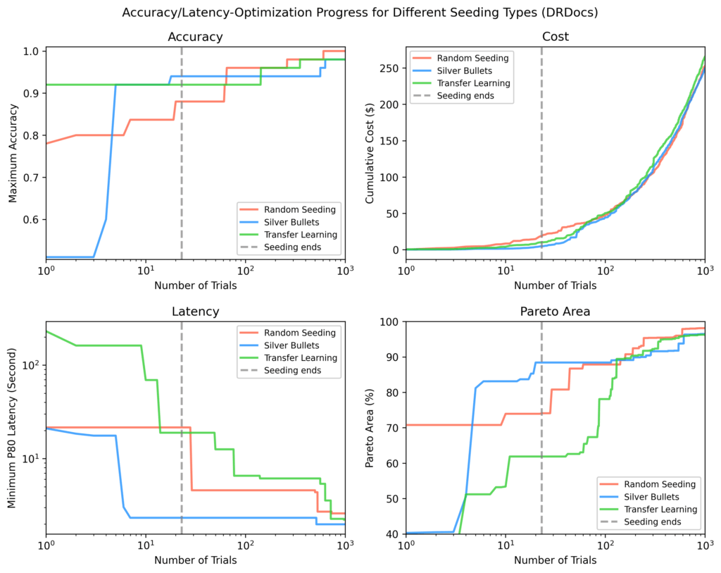
DRDocs
Similar to Bright Biology, silver bullets reached an 88% Pareto-area after seeding vs. 71% (transfer learning) and 62% (random).
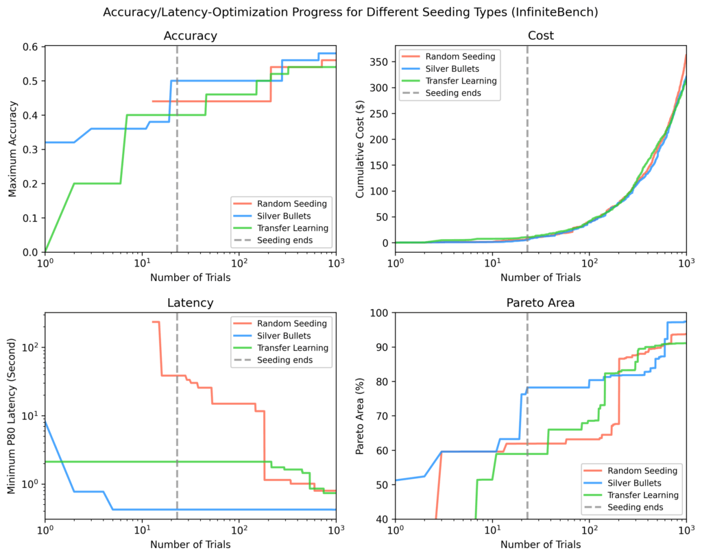
InfiniteBench
Other methods needed ~100 additional trials to match the silver bullet Pareto-area, and still didn’t match the fastest flows found via silver bullets by the end of ~1,000 trials.
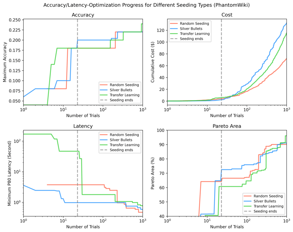
PhantomWiki
Silver bullets again performed best after seeding. This dataset showed the widest cost divergence. After ~70 trials, the silver bullet run briefly focused on more expensive flows.
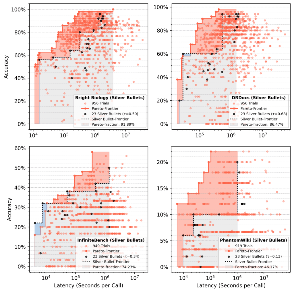
Pareto-fraction analysis
In runs seeded with silver bullets, the 23 silver bullet flows accounted for ~75% of the final Pareto-area after 1,000 trials, on average.
- Red area: Gains from optimization over initial silver bullet performance.
- Blue area: Silver bullet flows still dominating at the end.
Our takeaway
Seeding with silver bullets delivers consistently strong results and even outperforms transfer learning, despite that method pulling from a diverse set of historical Pareto-frontier flows.
For our two objectives (accuracy and latency), silver bullets always start with higher accuracy and lower latency than flows from other strategies.
In the long run, the TPE sampler reduces the initial advantage. Within a few hundred trials, results from all strategies often converge, which is expected since each should eventually find optimal flows.
So, do agentic flows exist that work well across many use cases? Yes — to a point:
- On average, a small set of silver bullets recovers about 75% of the Pareto-area from a full optimization.
- Performance varies by dataset, such as 92% recovery for Bright Biology compared to 46% for PhantomWiki.
Bottom line: silver bullets are an inexpensive and efficient way to approximate a full syftr run, but they are not a replacement. Their impact could grow with more training datasets or longer training optimizations.
Silver bullet parametrizations
We used the following:
LLMs
- microsoft/Phi-4-multimodal-instruct
- deepseek-ai/DeepSeek-R1-Distill-Llama-70B
- Qwen/Qwen2.5
- Qwen/Qwen3-32B
- google/gemma-3-27b-it
- nvidia/Llama-3_3-Nemotron-Super-49B
Embedding models
- BAAI/bge-small-en-v1.5
- thenlper/gte-large
- mixedbread-ai/mxbai-embed-large-v1
- sentence-transformers/all-MiniLM-L12-v2
- sentence-transformers/paraphrase-multilingual-mpnet-base-v2
- BAAI/bge-base-en-v1.5
- BAAI/bge-large-en-v1.5
- TencentBAC/Conan-embedding-v1
- Linq-AI-Research/Linq-Embed-Mistral
- Snowflake/snowflake-arctic-embed-l-v2.0
- BAAI/bge-multilingual-gemma2
Flow types
- vanilla RAG
- ReAct RAG agent
- Critique RAG agent
- Subquestion RAG
Here’s the full list of all 23 silver bullets, sorted from low accuracy / low latency to high accuracy / high latency: silver_bullets.json.
Try it yourself
Want to experiment with these parametrizations? Use the running_flows.ipynb notebook in our syftr repository — just make sure you have access to the models listed above.
For a deeper dive into syftr’s architecture and parameters, check out our technical paper or explore the codebase.
We’ll also be presenting this work at the International Conference on Automated Machine Learning (AutoML) in September 2025 in New York City.
The post Silver bullets: a shortcut to optimized agentic workflows appeared first on DataRobot.