Reinforcement learning has seen a great deal of success in solving complex decision making problems ranging from robotics to games to supply chain management to recommender systems. Despite their success, deep reinforcement learning algorithms can be exceptionally difficult to use, due to unstable training, sensitivity to hyperparameters, and generally unpredictable and poorly understood convergence properties. Multiple explanations, and corresponding solutions, have been proposed for improving the stability of such methods, and we have seen good progress over the last few years on these algorithms. In this blog post, we will dive deep into analyzing a central and underexplored reason behind some of the problems with the class of deep RL algorithms based on dynamic programming, which encompass the popular DQN and soft actor-critic (SAC) algorithms – the detrimental connection between data distributions and learned models.
Before diving deep into a description of this problem, let us quickly recap some of the main concepts in dynamic programming. Algorithms that apply dynamic programming in conjunction with function approximation are generally referred to as approximate dynamic programming (ADP) methods. ADP algorithms include some of the most popular, state-of-the-art RL methods such as variants of deep Q-networks (DQN) and soft actor-critic (SAC) algorithms. ADP methods based on Q-learning train action-value functions, $Q(s, a)$, via a Bellman backup. In practice, this corresponds to training a parametric function, $Q_\theta(s, a)$, by minimizing the mean squared difference to a backup estimate of the Q-function, defined as:
$\mathcal{B}^*Q(s, a) = r(s, a) + \gamma \mathbb{E}_{s’|s, a} [\max_{a’} \bar{Q}(s’, a’)],$
where $\bar{Q}$ denotes a previous instance of the original Q-function, $Q_\theta$, and is commonly referred to as a target network. This update is summarized in the equation below.
An analogous update is also used for actor-critic methods that also maintain an explicitly parametrized policy, $\pi_\phi(a|s)$, alongside a Q-function. Such an update typically replaces $\max_{a’}$ with an expectation under the policy, $\mathbb{E}_{a’ \sim \pi_\phi}$. We shall use the $\max_{a’}$ version for consistency throughout, however, the actor-critic version follows analogously. These ADP methods aim at learning the optimal value function, $Q^*$, by applying the Bellman backup iteratively untill convergence.
A central factor that affects the performance of ADP algorithms is the choice of the training data-distribution, $\mathcal{D}$, as shown in the equation above. The choice of $\mathcal{D}$ is an integral component of the backup, and it affects solutions obtained via ADP methods, especially since function approximation is involved. Unlike tabular settings, function approximation causes the learned Q function to depend on the choice of data distribution $\mathcal{D}$, thereby affecting the dynamics of the learning process. We show that on-policy exploration induces distributions $\mathcal{D}$ such that training Q-functions under $\mathcal{D}$ may fail to correct systematic errors in the Q-function, even if Bellman error is minimized as much as possible – a phenomenon that we refer to as an absence of corrective feedback.
Corrective Feedback and Why it is Absent in ADP
What is corrective feedback formally? How do we determine if it is present or absent in ADP methods? In order to build intuition, we first present a simple contextual bandit (one step RL) example, where the Q-function is trained to match $Q^*$ via supervised updates, without bootstrapping. This enjoys corrective feedback, and we then contrast it with ADP methods, which do not. In this example, the goal is to learn the optimal value function $Q^*(s, a)$, which, is equal to the reward $r(s, a)$. At iteration $k$, the algorithm minimizes the estimation error of the Q-function:
$\mathcal{L}(Q) = \mathbb{E}_{s \sim \beta(s), a \sim \pi_k(a|s)}[|Q_k(s, a) – Q^*(s, a)|].$
Using an $\varepsilon$-greedy or Boltzmann policy for exploration, denoted by $\pi_k$, gives rise to a hard negative mining phenomenon – the policy chooses precisely those actions that correspond to possibly over-estimated Q-values for each state $s$ and observes the corresponding, $r(s, a)$ or $Q^*(s, a)$, as a result. Then, minimizing $\mathcal{L}(Q)$, on samples collected this way corrects errors in the Q-function, as $Q_k(s, a)$ is pushed closer to match $Q^*(s, a)$ for actions $a$ with incorrectly high Q-values, correcting precisely the Q-values which may cause sub-optimal performance. This constructive interaction between online data collection and error correction – where the induced online data distribution corrects errors in the value function – is what we refer to as corrective feedback.
In contrast, we will demonstrate that ADP methods that rely on previous Q-functions to generate targets for training the current Q-function, may not benefit from corrective feedback. This difference between bandits and ADP happens because the target values are computed by applying a Bellman backup on the previous Q-function, (target value), rather than the optimal $Q^*$, so, errors in $\bar{Q}$, at the next states can result in incorrect Q-value targets at the current state. No matter how often the current transition is observed, or how accurately Bellman errors are minimized, the error in the Q-value with respect to the optimal Q-function, $|Q – Q^*|$, at this state is not reduced. Furthermore, in order to obtain correct target values, we need to ensure that values at state-action pairs occurring at the tail ends of the data distribution $\mathcal{D}$, which are primary causes of errors in Q-values at other states, are correct. However, as we will show via a simple didactic example, that this correction process may be extremely slow and may not occur, mainly because of undesirable generalization effects of the function approximator.
Let’s consider a didactic example of a tree-structured deterministic MDP with 7 states and 2 actions, $a_1$ and $a_2$, at each state.

Figure 1: Run of an ADP algorithm with on-policy data collection. Boxed nodes and circled nodes denote groups of states aliased by function approximation — values of these nodes are affected due to parameter sharing and function approximation.
A run of an ADP algorithm that chooses the current on-policy state-action marginal as $\mathcal{D}$ on this tree MDP is shown in Figure 1. Thus, the Bellman error at a state is minimized in proportion to the frequency of occurrence of that state in the policy state-action marginal. Since the leaf node states are the least frequent in this on-policy marginal distribution (due to the discounting), the Bellman backup is unable to correct errors in Q-values at such leaf nodes, due to their low frequency and aliasing with other states arising due to function approximation. Using incorrect Q-values at the leaf nodes to generate targets for other nodes in the tree, just gives rise to incorrect values, even if Bellman error is fully minimized at those states. Thus, most of the Bellman updates do not actually bring Q-values at the states of the MDP closer to $Q^*$, since the primary cause of incorrect target values isn’t corrected.
This observation is surprising, since it demonstrates how the choice of an online distribution coupled with function approximation might actually learn incorrect Q-values. On the other hand, a scheme that chooses to update states level by level progressively (Figure 2), ensuring that target values used at any iteration of learning are correct, very easily learns correct Q-values in this example.

Figure 2: Run of an ADP algorithm with an oracle distribution, that updates states level-by level, progressing through the tree from the leaves to the root. Even in the presence of function approximation, selecting the right set of nodes for updates gives rise to correct Q-values.
Consequences of Absent Corrective Feedback
Now, one might ask if an absence of corrective feedback occurs in practice, beyond a simple didactic example and whether it hurts in practical problems. Since visualizing the dynamics of the learning process is hard in practical problems as we did for the didactic example, we instead devise a metric that quantifies our intuition for corrective feedback. This metric, what we call value error, is given by:
Increasing values of imply that the algorithm is pushing Q-values farther away from $Q^*$, which means that corrective feedback is absent, if this happens over a number of iterations. On the other hand, decreasing values of $\mathcal{E}_k$ implies that the algorithm is continuously improving its estimate of $Q$, by moving it towards $Q^*$ with each iteration, indicating the presence of corrective feedback.
Observe in Figure 3, that ADP methods can suffer from prolonged periods where this global measure of error in the Q-function, $\mathcal{E}_k$, is increasing or fluctuating, and the corresponding returns degrade or stagnate, implying an absence of corrective feedback.

Figure 3: Consequences of absent corrective feedback, including (a) sub-optimal convergence, (b) instability in learning and (c) inability to learn with sparse rewards.
In particular, we describe three different consequences of an absence of corrective feedback:
-
Convergence to suboptimal Q-functions. We find that on-policy sampling can cause ADP to converge to a suboptimal solution, even in the absence of sampling error. Figure 3(a) shows that the value error $\mathcal{E}_k<$ rapidly decreases initially, and eventually converges to a value significantly greater than 0, from which the learning process never recovers.
-
Instability in the learning process. We observe that ADP with replay buffers can be unstable. For instance, the algorithm is prone to degradation even if the latest policy obtains returns that are very close to the optimal return in Figure 3(b).
-
Inability to learn with low signal-to-noise ratio. Absence of corrective feedback can also prevent ADP algorithms from learning quickly in scenarios with low signal-to-noise ratio, such as tasks with sparse/noisy rewards as shown in Figure 3(c). Note that this is not an exploration issue, since all transitions in the MDP are provided to the algorithm in this experiment.
Inducing Maximal Corrective Feedback via Distribution Correction
Now that we have defined corrective feedback and gone over some detrimental consequences an absence of it can have on the learning process of an ADP algorithm, what might be some ways to fix this problem? To recap, an absence of corrective feedback occurs when ADP algorithms naively use the on-policy or replay buffer distributions for training Q-functions. One way to prevent this problem is by computing an “optimal” data distribution that provides maximal corrective feedback, and train Q-functions using this distribution? This way we can ensure that the ADP algorithm always enjoys corrective feedback, and hence makes steady learning progress. The strategy we used in our work is to compute this optimal distribution and then perform a weighted Bellman update that re-weights the data distribution in the replay buffer to this optimal distribution (in practice, a tractable approximation is required, as we will see) via importance sampling based techniques.
We will not go into the full details of our derivation in this article, however, we mention the optimization problem used to obtain a form for this optimal distribution and encourage readers interested in the theory to checkout Section 4 in our paper. In this optimization problem, our goal is to minimize a measure of corrective feedback, given by value error $\mathcal{E}_k$, with respect to the distribution $p_k$ used for Bellman error minimization, at every iteration $k$. This gives rise to the following problem:
$\min _{p_{k}} \; \mathbb{E}_{d^{\pi_{k}}}[|Q_{k}-Q^{*}|]$
$\text { s.t. }\;\; Q_{k}=\arg \min _{Q} \mathbb{E}_{p_{k}}\left[\left(Q-\mathcal{B}^{*} Q_{k-1}\right)^{2}\right]$
We show in our paper that the solution of this optimization problem, that we refer to as the optimal distribution, $p_k^*$, is given by:
$p_{k}^*(s, a) \propto \exp \left(-\left|Q_{k}-Q^{*}\right|(s, a)\right) \frac{\left|Q_{k}-\mathcal{B}^{*} Q_{k-1}\right|(s, a)}{\lambda^{*}}$
By simplifying this expression, we obtain a practically viable expression for weights, $w_k$, at any iteration $k$ that can be used to re-weight the data distribution:
$w_{k}(s, a) \propto \exp \left(-\frac{\gamma \mathbb{E}_{s’|s, a} \mathbb{E}_{a’ \sim \pi_\phi(\cdot|s’)} \Delta_{k-1}(s’, a’)}{\tau}\right)$
where $\Delta_k$ is the accumulated Bellman error over iterations, and it satisfies a convenient recursion making it amenable to practical implementations,
$\Delta_{k}(s, a) =\left|Q_{k}-\mathcal{B}^{*} Q_{k-1}\right|(s, a) +\gamma \mathbb{E}_{s’|s, a} \mathbb{E}_{a’ \sim \pi_\phi(\cdot|s’)} \Delta_{k-1}(s’, a’)$
and $\pi_\phi$ is the Boltzmann or $\varepsilon-$greedy policy corresponding to the current Q function.
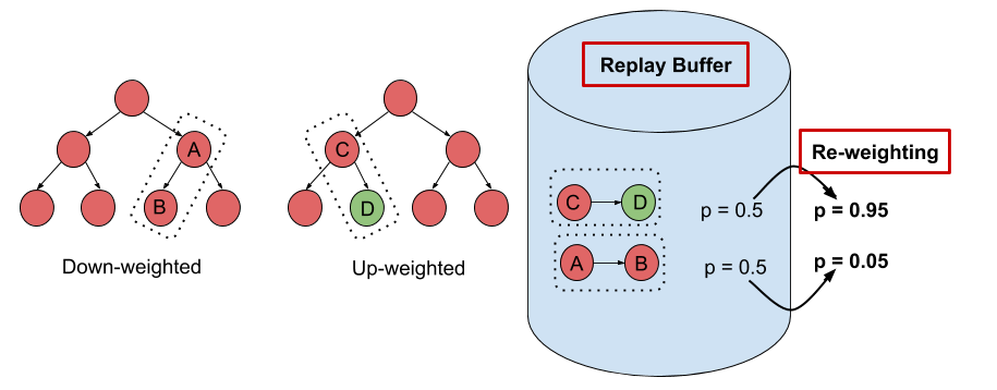
What does this expression for $w_k$ intuitively correspond to? Observe that the term appearing in the exponent in the expression for $w_k$ corresponds to the accumulated Bellman error in the target values. Our choice of $w_k$, thus, basically down-weights transitions with highly incorrect target values. This technique falls into a broader class of abstention based techniques that are common in supervised learning settings with noisy labels, where down-weighting datapoints (transitions here) with errorful labels (target values here) can boost generalization and correctness properties of the learned model.

Figure 4: Schematic of the DisCor algorithm. Transitions with errorful target values are downweighted.
Why does our choice of $\Delta_k$, i.e. the sum of accumulated Bellman errors suffice? This is because this value $\Delta_k$ accounts for how error is propagated in ADP methods. Bellman errors, $|Q_k – \mathcal{B}^*Q_{k-1}|$ are propagated under the current policy $\pi_{k-1}$, and then discounted when computing target values for updates in ADP. $\Delta_k$ captures exactly this, and therefore, using this estimate in our weights suffices.
Our practical algorithm, that we refer to as DisCor (Distribution Correction), is identical to conventional ADP methods like Q-learning, with the exception that it performs a weighted Bellman backup – it assigns a weight $w_k(s,a)$ to a transition, $(s, a, r, s’)$ and performs a Bellman backup weighted by these weights, as shown below.
We depict the general principle in the schematic diagram shown in Figure 4.
We finally present some results that demonstrate the efficacy of our method, DisCor, in practical scenarios. Since DisCor only modifies the chosen distribution for the Bellman update, it can be applied on top of any standard ADP algorithm including soft actor-critic (SAC) or deep Q-network (DQN). Our paper presents results for a number of tasks spanning a wide variety of settings including robotic manipulation tasks, multi-task reinforcement learning tasks, learning with stochastic and noisy rewards, and Atari games. In this blog post, we present two of these results from robotic manipulation and multi-task RL.
-
Robotic manipulation tasks. On six challenging benchmark tasks from the MetaWorld suite, we observe that DisCor when combined with SAC greatly outperforms prior state-of-the-art RL algorithms such as soft actor-critic (SAC) and prioritized experience replay (PER) which is a prior method that prioritizes states with high Bellman error during training. Note that DisCor usually starts learning earlier than other methods compared to. DisCor outperforms vanilla SAC by a factor of about 50% on average, in terms of success rate on these tasks.

-
Multi-task reinforcement learning. We also present certain results on the Multi-task 10 (MT10) and Multi-task 50 (MT50) benchmarks from the Meta-world suite. The goal here is to learn a single policy that can solve a number of (10 or 50, respectively) different manipulation tasks that share common structure. We note that DisCor outperforms, state-of-the-art SAC algorithm on both of these benchmarks by a wide margin (for e.g. 50% on MT10, success rate). Unlike the learning process of SAC that tends to plateau over the course of learning, we observe that DisCor always exhibits a non-zero gradient for the learning process, until it converges.

In our paper, we also perform evaluations on other domains such as Atari games and OpenAI gym benchmarks, and we encourage the readers to check those out. We also perform an analysis of the method on tabular domains, understanding different aspects of the method.
Perspectives, Future Work and Open Problems
Some of our and other prior work has highlighted the impact of the data distribution on the performance of ADP algorithms, We observed in another prior work that in contrast to the intuitive belief about the efficacy of online Q-learning with on-policy data collection, Q-learning with a uniform distribution over states and actions seemed to perform best. Obtaining a uniform distribution over state-action tuples during training is not possible in RL, unless all states and actions are observed at least once, which may not be the case in a number of scenarios. We might also ask the question about whether the uniform distribution is the best choice that can be used in an RL setting? The form of the optimal distribution derived in Section 4 of our paper, is a potentially better choice since it is customized to the MDP under consideration.
Furthermore, in the domain of purely offline reinforcement learning, studied in our prior work and some other works, such as this and this, we observe that the data distribution is again a central feature, where backing up out-of-distribution actions and the inability to try these actions out in the environment to obtain answers to counterfactual queries, can cause error accumulation and backups to diverge. However, in this work, we demonstrate a somewhat counterintuitive finding: even with on-policy data collection, where the algorithm, in principle, can evaluate all forms of counterfactual queries, the algorithm may not obtain a steady learning progress, due to an undesirable interaction between the data distribution and generalization effects of the function approximator.

What might be a few promising directions to pursue in future work?
Formal analysis of learning dynamics: While our study is an initial foray into the role that data distributions play in the learning dynamics of ADP algorithms, this motivates a significantly deeper direction of future study. We need to answer questions related to how deep neural network based function approximators actually behave, which are behind these ADP methods, in order to get them to enjoy corrective feedback.
Re-weighting to supplement exploration in RL problems: Our work depicts the promise of re-weighting techniques as a practically simple replacement for altering entire exploration strategies. We believe that re-weighting techniques are very promising as a general tool in our toolkit to develop RL algorithms. In an online RL setting, re-weighting can help remove the some of the burden off exploration algorithms, and can thus, potentially help us employ complex exploration strategies in RL algorithms.
More generally, we would like to make a case of analyzing effects of data distribution more deeply in the context of deep RL algorithms. It is well known that narrow distributions can lead to brittle solutions in supervised learning that also do not generalize. What is the corresponding analogue in reinforcement learning? Distributional robustness style techniques have been used in supervised learning to guarantee a uniformly convergent learning process, but it still remains unclear how to apply these in an RL with function approximation setting. Part of the reason is that the theory of RL often derives from tabular settings, where distributions do not hamper the learning process to the extent they do with function approximation. However, as we showed in this work, choosing the right distribution may lead to significant gains in deep RL methods, and therefore, we believe, that this issue should be studied in more detail.
This blog post is based on our recent paper:
- DisCor: Corrective Feedback in Reinforcement Learning via Distribution Correction
Aviral Kumar, Abhishek Gupta, Sergey Levine
arXiv
We thank Sergey Levine and Marvin Zhang for their valuable feedback on this blog post.
This article was initially published on the BAIR blog, and appears here with the authors’ permission.