All posts by Stefan Hackmann

TL;DR

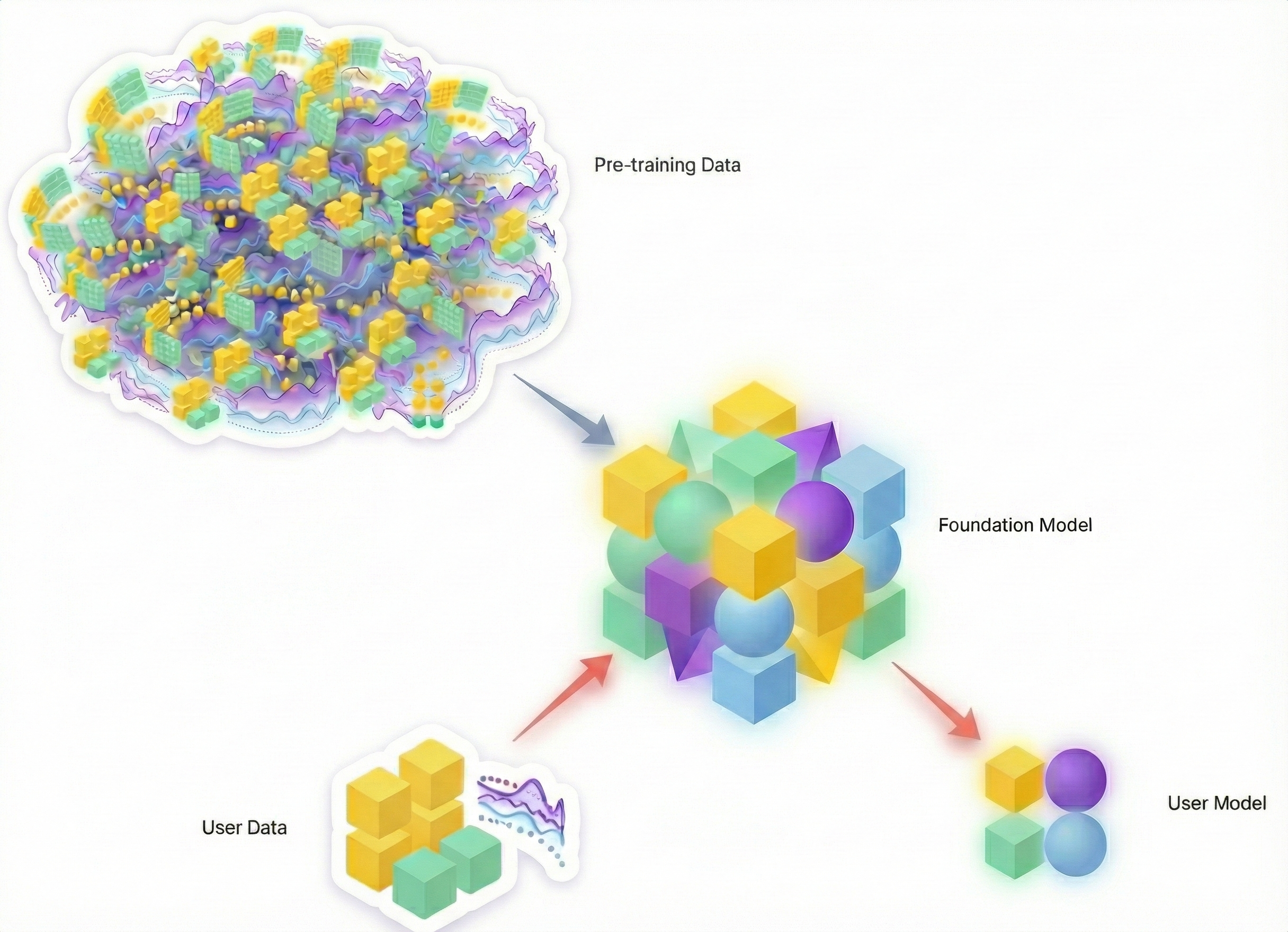
JointFM is the first AI foundation model for zero-shot joint distributional forecasting in multivariate time-series systems. By generating coherent future scenarios in milliseconds, it enables real-time portfolio decision-making without the lag of traditional numerical simulations. JointFM represents a paradigm shift in quantitative modeling: trained on an infinite stream of dynamics from synthetic stochastic differential equations (SDEs), JointFM acts as your digital quant.

Setting the stage: why quantitative modeling needs a new approach

Modeling complex systems has traditionally required a painful trade-off. Classical quant methods (like correlation copulas or coupled SDEs) offer high mathematical fidelity but are rigid, slow, and expensive. They often require specialized teams to rebuild models whenever the market regime or asset mix changes. Conversely, existing time-series foundation models offer speed and flexibility but are single-target, missing the critical cross-variable dependencies that define systemic risk.

JointFM is your “digital quant“ to bridge this gap. Trained on an infinite stream of synthetic stochastic differential equations (SDEs), it learns the universal physics of time-series dynamics, making it truly domain-agnostic. Whether for a power grid or a stock portfolio, it predicts the full joint probability distribution of the system in milliseconds. This is the foundation of instant decision-making in highly complex setups and is fast enough to integrate with agents for ad-hoc business decisions.

In this project, we demonstrate its power in quantitative finance, building on NVIDIA’s quantitative portfolio optimization blueprint. JointFM enables instant portfolio optimization (IPO), replacing brittle overnight batch processes with a digital quant that can rebalance portfolios in real time and adapt to new assets or market conditions without retraining.

Key takeaways 

• The first zero-shot foundation model for joint distributions: JointFM predicts full multivariate distributions out of the box, capturing correlations and tail risk.
  
• Instant simulation at portfolio scale: thousands of coherent future scenarios are generated in milliseconds, independent of portfolio complexity, enabling real-time decision-making and AI agent integration.
  
• Matches the risk-adjusted returns of the classical benchmark: across 200 controlled synthetic trials, JointFM achieved equal risk-adjusted performance.
  
• Pre-trained on synthetic stochastic processes: by learning from millions of generated dynamics, JointFM generalizes to new assets and market conditions without retraining.
  
• From financial modeling to financial AI: JointFM replaces classical pipelines with a scalable, domain-agnostic foundation model.

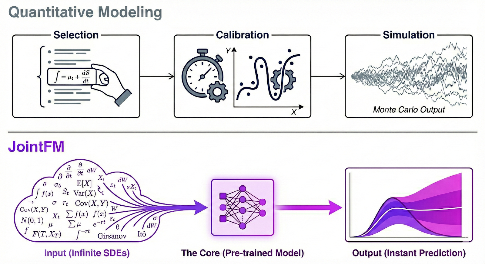
The core challenge: speed, fidelity, and flexibility

In quantitative finance, portfolio managers have long faced a customized trilemma:

1. Fast but flawed: models like Geometric Brownian Motion (GBM) are computationally cheap but assume normal distributions and constant correlations. They fail spectacularly during market crashes, when assets become highly correlated and fat tails appear.
2. Accurate but slow: heavy Monte Carlo simulations with complex copulas or regime-switching variations capture reality better but take much longer to calibrate and run, making them impractical when you need to rebalance your portfolio on short notice.
3. Rigid and expensive: developing high-fidelity models requires specialized quantitative modeling teams, significant time, and money. Worse, these models are often brittle; when the market regime shifts or you want to swap asset classes, you often need to start modeling again from scratch.

Enter JointFM: a foundation model for joint distributions

JointFM changes the game by “skipping” the modeling step. Instead of fitting parameters for each time series daily, JointFM is a pre-trained model that generalizes to unseen data out of the box. While we apply it here to financial markets, the model itself is domain-agnostic. It learns the language of stochastic processes, not just stock tickers.

The innovation

Until now, modeling joint distributions required significant compromises. You could define complex systems of SDEs (mathematically difficult), fit specialized classical models to specific datasets (slow and requiring retraining), or use copulas (bespoke and rigid). 

None of these are zero-shot. 

On the other hand, existing foundation models are zero-shot but fail to capture cross-variable dependencies. JointFM is the first to bridge this divide, offering the scale and zero-shot speed of a foundation model with the mathematical depth of a rigorous joint probability framework.

This zero-shot capability solves the rigidity problem. Facing a new market situation where you don’t know the underlying dynamics? Want to swap difficult-to-model assets instantly? JointFM works just the same. Because it has learned to predict future joint distributions from almost any dynamic during its diverse pre-training, it serves as the best possible starting point for unknown environments without the need for a dedicated quant team to build a new model from scratch.

Key capabilities

• Joint distributional forecasting: unlike standard univariate time-series models that predict marginal probabilities for one variable at a time, JointFM explicitly models the full multivariate distribution of all variables simultaneously. In finance, this is critical for diversification. You cannot optimize a portfolio without understanding how assets move together.
• Zero-shot inference: no training required on the user’s data. The model has already “seen it all” during pre-training.
• Scenario slicing: the model can condition predictions on exogenous variables (e.g., “Show me the distribution of variables if an external factor rises”).

If you want to read more about time-series and tabular foundation models, have a look at this article on the brewing GenAI data science revolution, which gives an introduction to the field and explains why a model like JointFM is the next logical step.

Under the hood: architecture & speed

JointFM leverages a specialized transformer-based architecture designed to handle the unique high-dimensional constraints of multivariate time series.

1. Efficient high-dimensional context

To model portfolios with many assets over long history windows, JointFM moves beyond the quadratic complexity of standard attention mechanisms. Like other single-target models, JointFM employs a factored attention strategy that efficiently decouples temporal dynamics from cross-variable dependencies. This allows the model to scale linearly with the complexity of the portfolio, processing hundreds of assets without becoming a computational bottleneck.

2. Heavy-tailed distributional heads

Real-world data is rarely normal; it often exhibits heavy tails and skewness. JointFM utilizes a flexible output layer capable of parameterizing robust, fat-tailed multivariate distributions. This enables the model to naturally capture the probability of extreme events (“black swans”) that are critical for accurate risk assessment.

3. Parallel decoding for instant results

Speed is the central enabler of instant portfolio optimization. While also supporting an autoregressive mode, the model architecture is optimized for parallel decoding, allowing it to predict all future horizons simultaneously in a single forward pass. This capability—distinct from the slow, sequential generation of traditional autoregressive models—enables the generation of thousands of coherent market scenarios in milliseconds on a GPU.

The secret sauce: synthetic pre-training

Why does JointFM work so well on real data without seeing it? Synthetic pre-training.

Real historical data is often finite, noisy, and regime-specific. To build a truly general foundation model, JointFM is trained on an infinite curriculum of synthetic data generated by a flexible engine. We lead with finance because of its notoriously complex dynamics and its significance as a benchmark application for our work. However, while the domain is specialized, the core technology is universal.

1. SDESampler: this is the core of the system. It generates complex stochastic differential equations (SDEs) with jumps, complex drifts, path-dependent memory, and regimes. It is designed to simulate any continuous-time system with stochastic components.
2. FinanceSampler: to address the wide array of financial asset classes, we developed a specialized sampler that works alongside our generic engine. For the purpose of this simple benchmark comparison, we limited the selection to the most fundamental asset classes: equities, precious metals, and foreign exchange (FX).
3. Custom extensibility: while we focused on finance, the same architecture allows us to build other samplers (e.g., for weather, energy, or sensor data) to target different domains.

This approach exposes the model to millions of regimes, ensuring it learns the fundamental physics of time-series dynamics rather than just memorizing historical patterns.

Performance evaluation: benchmarking against classical methods

We compared JointFM-optimized portfolios against classical Geometric Brownian Motion (GBM)-optimized portfolios as a simple baseline. Read about our experiment setup below, followed by the results.

Experimental setup 

Our portfolio optimization setup, while drawing inspiration from the NVIDIA blueprint, incorporates a few key differences. Similar to the blueprint, we utilize the same GBM simulation and Mean-CVaR optimization but use JointFM as an alternative scenario generator and our FinanceSampler as well as S&P 500 stock prices as input data.

1. Input:
   • Synthetic reality: We generate complex asset histories using the FinanceSampler (SDEs with stochastic volatility, correlated drifts, etc.). This ensures we have a ground-truth multiverse of future possibilities for objective evaluation.
   • Real data (secondary check): we also plug in real historical returns (S&P 500) to confirm the model generalizes to the noisy, imperfect real world.
     
2. Inference:
   • GBM—classical SDE calibration and path generation from the NVIDIA blueprint.
   • JointFM—trained on similar but not identical synthetic physics—generates 10,000+ plausible future return scenarios in milliseconds. It effectively acts as a “future oracle” that intimately understands the statistical laws governing the assets.
     
3. Risk optimization:
   • A Mean-CVaR (conditional value at risk) optimizer solves for the portfolio weights that maximize risk-adjusted returns (balancing expected return against tail risk).
     
4. Execution and scoring:
   • We deploy the optimal weights into the known future:
     1. Synthetic ground-truth data provides thousands of scenarios for evaluation per experiment step.
     2. Real data has one known future for every historical experiment.

Speed: simulate the future instantly

JointFM generates scenarios in milliseconds, even orders of magnitude faster than relatively simple geometric Brownian motion (GBM) simulations.

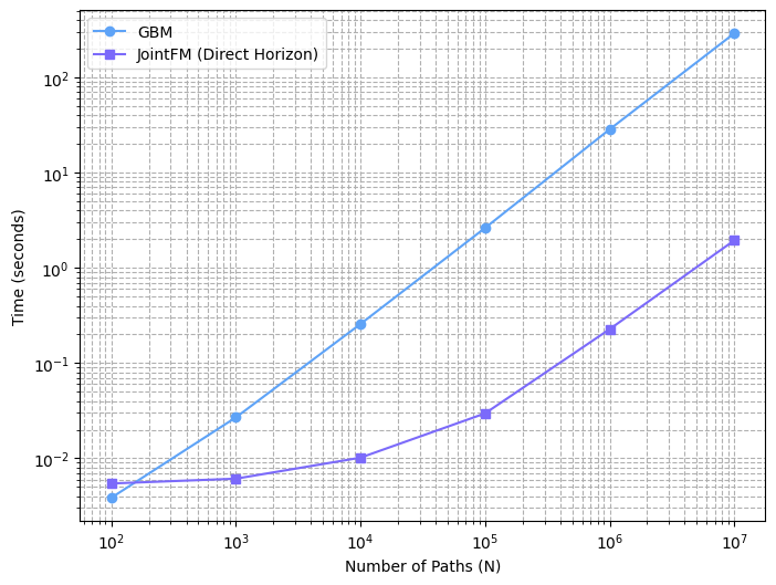
This architectural advantage enables timely reactions to market changes and makes it practical to integrate sophisticated simulation and portfolio optimization directly into an AI agent. As a result, investors can explore and discuss investment decisions in real time without additional operational overhead.

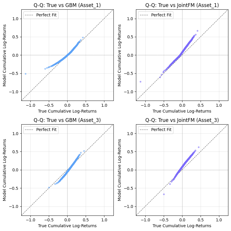
Performance on marginals: looking at one asset at a time

JointFM recovers the marginal distributions of complex assets to some extent. Below we show the Q-Q (quantile-quantile) plot for each percentile and two random assets of one anecdotal simulation/prediction. 

While we clearly aim to further improve the marginal predictability, there are two things here that are critical to understand:

1. The dynamics of financial assets are notoriously hard to predict (here 63 days ahead).  
2. Being good at making marginal predictions alone does not help with risk management very much. It is critical to capture asset correlations as well.

Directly comparing high-dimensional joint probability distributions is impractical. Instead, we present a simple demonstration showing that JointFM provides consistent and reliable predictions for portfolio optimization, matching or exceeding the baseline quantitative method.

Portfolio evaluation (synthetic ground truth)

To rigorously evaluate performance, we conducted 200 repeated portfolio optimization trials using synthetic data in which the true future joint distributions are known. This controlled setting allows us to directly compare JointFM-generated portfolios and our baseline against the ground-truth optimum.

The results

• Simple returns: JointFM portfolios achieved 1.17% higher returns on average.
• Risk-adjusted returns: the Sharpe ratio is practically the same. JointFM shows a slightly better risk-adjusted return.

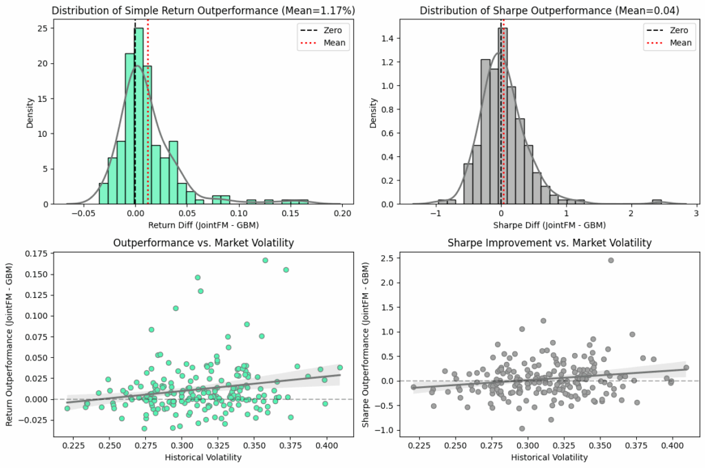
On the synthetic oracle data, the JointFM portfolio has a 1.17% higher return on average but at a roughly identical risk-adjusted return (Sharpe ratio), which means that the outperformance resulted from more risk-taking. Given its roughly identical performance in terms of risk-adjusted return, which is the more important metric, our first version of JointFM emerges as a fast, cheap, flexible, and simple drop-in alternative to the baseline approach.

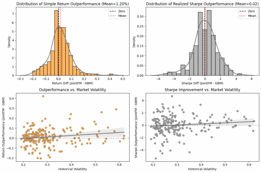
Real-world sanity check

Addressing the potential concern that our model is only good at solving the specific synthetic problems it was trained on, we validated the approach on real S&P 500 data (Yahoo Finance). We randomly sampled 10 assets over 200 different time periods out of a universe of 391 different stocks from the S&P 500. 

The results

JointFM-portfolios, similar to their performance on the synthetic test datasets, showed a higher simple return. Their risk-adjusted return is approximately the same as the comparison, slightly outperforming it. This confirms that the model has learned generalizable rules of volatility and correlation, not just memorized a specific set of data-generating processes.

Wrapping up: instant portfolio optimization

By replacing rigid statistical assumptions with a flexible, pre-trained foundation model, JointFM enables a new class of trading and risk management agents. These agents don’t just react to price changes; they instantly re-simulate the future multiverse to find the best path forward. JointFM significantly accelerates inference by front-loading the extensive scientific modeling into the training stage. This allows for near-instantaneous inference execution.

This represents a shift from financial modeling (fitting equations) to financial AI (using foundation models), offering both the speed required for modern markets and the depth required for survival.

Should you have any questions, please contact us at research@datarobot.com.

The post The digital quant: instant portfolio optimization with JointFM appeared first on DataRobot.

If you lead an enterprise data science team or a quantitative research unit today, you likely feel like you are living in two parallel universes.

In one universe, you have the “GenAI” explosion. Chatbots now write code and create art, and boardrooms are obsessed with how large language models (LLMs) will change the world. In the other universe, you have your day job: the “serious” work of predicting churn, forecasting demand, and detecting fraud using structured, tabular data. 

For years, these two universes have felt completely separate. You might even feel that the GenAI hype rocketship has left your core business data standing on the platform.

But that separation is an illusion, and it is disappearing fast.

From chatbots to forecasts: GenAI arrives at tabular and time-series modeling

Whether you are a skeptic or a true believer, you have most certainly interacted with a transformer model to draft an email or a diffusion model to generate an image. But while the world was focused on text and pixels, the same underlying architectures have been quietly learning a different language: the language of numbers, time, and tabular patterns. 

Take for instance SAP-RPT-1 and LaTable. The first uses a transformer architecture, and the second is a diffusion model; both are used for tabular data prediction.

We are witnessing the emergence of data science foundation models.

These are not just incremental improvements to the predictive models you know. They represent a paradigm shift. Just as LLMs can “zero-shot” a translation task they weren’t explicitly trained for, these new models can look at a sequence of data, for example, sales figures or server logs, and generate forecasts without the traditional, labor-intensive training pipeline.

The pace of innovation here is staggering. By our count, since the beginning of 2025 alone, we have seen at least 14 major releases of foundation models specifically designed for tabular and time-series data. This includes impressive work from the teams behind Chronos-2, TiRex, Moirai-2, TabPFN-2.5, and TempoPFN (using SDEs for data generation), to name just a few frontier models.

Models have become model-producing factories

Traditionally, machine learning models were treated as static artifacts: trained once on historical data and then deployed to produce predictions.

That framing no longer holds. Increasingly, modern models behave less like predictors and more like model-generating systems, capable of producing new, situation-specific representations on demand. 

We are moving toward a future where you won’t just ask a model for a single point prediction; you will ask a foundation model to generate a bespoke statistical representation—effectively a mini-model—tailored to the specific situation at hand. 

The revolution isn’t coming; it’s already brewing in the research labs. The question now is: why isn’t it in your production pipeline yet?

The reality check: hallucinations and trend lines

If you’ve scrolled through the endless examples of grotesque LLM hallucinations online, including lawyers citing fake cases and chatbots inventing historical events, the thought of that chaotic energy infiltrating your pristine corporate forecasts is enough to keep you awake at night.

Your concerns are entirely justified.

Classical machine learning is the conservative choice for now

While the new wave of data science foundation models (our collective term for tabular and time-series foundation models) is promising, it is still very much in the early days. 

Yes, model providers can currently claim top positions on academic benchmarks: all top-performing models on the time-series forecasting leaderboard GIFT-Eval and the tabular data leaderboard TabArena are now foundation models or agentic wrappers of foundation models. But in practice? The reality is that some of these “top-notch” models currently struggle to identify even the most basic trend lines in raw data. 

They can handle complexity, but sometimes trip over the basics that a simple regression would nail it–check out the honest ablation studies in the TabPFN v2 paper, for instance.

Why we remain confident: the case for foundation models

While these models still face early limitations, there are compelling reasons to believe in their long-term potential. We have already discussed their ability to react instantly to user input, a core requirement for any system operating in the age of agentic AI. More fundamentally, they can draw on a practically limitless reservoir of prior information.

Think about it: who has a better chance at solving a complex prediction problem?

• Option A: A classical model that knows your data, but only your data. It starts from zero every time, blind to the rest of the world.

• Option B: A foundation model that has been trained on a mind-boggling number of relevant problems across industries, decades, and modalities—often augmented by vast amounts of synthetic data—and is then exposed to your specific situation.

Classical machine learning models (like XGBoost or ARIMA) do not suffer from the “hallucinations” of early-stage GenAI, but they also do not come with a “helping prior.” They cannot transfer wisdom from one domain to another. 

The bet we are making, and the bet the industry is moving toward, is that eventually, the model with the “world’s experience” (the prior) will outperform the model that is learning in isolation.

The missing link: solving for reality, not leaderboards

Data science foundation models have a shot at becoming the next massive shift in AI. But for that to happen, we need to move the goalposts. Right now, what researchers are building and what businesses actually need remains disconnected. 

Leading tech companies and academic labs are currently locked in an arms race for numerical precision, laser-focused on topping prediction leaderboards just in time for the next major AI conference. Meanwhile, they are paying relatively little attention to solving complex, real-world problems, which, ironically, pose the toughest scientific challenges.

The blind spot: interconnected complexity

Here is the crux of the problem: none of the current top-tier foundation models are designed to predict the joint probability distributions of several dependent targets.

That sounds technical, but the business implication is massive. In the real world, variables rarely move in isolation.

• City Planning: You cannot predict traffic flow on Main Street without understanding how it impacts (and is impacted by) the flow on 5th Avenue.
• Supply Chain: Demand for Product A often cannibalizes demand for Product B.
• Finance: Take portfolio risk. To understand true market exposure, a portfolio manager doesn’t simply calculate the worst-case scenario for every instrument in isolation. Instead, they run joint simulations. You cannot just sum up individual risks; you need a model that understands how assets move together.

The world is a messy, tangled web of dependencies. Current foundation models tend to treat it like a series of isolated textbook problems. Until these models can grasp that complexity, outputting a model that captures how variables dance together, they won’t replace existing solutions.

So, for the moment, your manual workflows are safe. But mistaking this temporary gap for a permanent safety net could be a grave mistake. 

Today’s deep learning limits are tomorrow’s solved engineering problems

The missing pieces, such as modeling complex joint distributions, are not impossible laws of physics; they are simply the next engineering hurdles on the roadmap. 

If the speed of 2025 has taught us anything, it is that “impossible” engineering hurdles have a habit of vanishing overnight. The moment these specific issues are addressed, the capability curve won’t just inch upward. It will spike.

Conclusion: the tipping point is closer than it appears

Despite the current gaps, the trajectory is clear and the clock is ticking. The wall between “predictive” and “generative” AI is actively crumbling.

We are rapidly moving toward a future where we don’t just train models on historical data; we consult foundation models that possess the “priors” of a thousand industries. We are heading toward a unified data science landscape where the output isn’t just a number, but a bespoke, sophisticated model generated on the fly.

The revolution is not waiting for perfection. It is iterating toward it at breakneck speed. The leaders who recognize this shift and begin treating GenAI as a serious tool for structured data before a perfect model reaches the market will be the ones who define the next decade of data science. The rest will be playing catch-up in a game that has already changed.

We are actively researching these frontiers at DataRobot to bridge the gap between generative capabilities and predictive precision. This is just the start of the conversation. Stay tuned—we look forward to sharing our insights and progress with you soon. 

In the meantime, you can learn more about DataRobot and explore the platform with a free trial. 

The post The brewing GenAI data science revolution appeared first on DataRobot.