By Sylvia Herbert, David Fridovich-Keil, and Claire Tomlin

The Problem: Fast and Safe Motion Planning

Real time autonomous motion planning and navigation is hard, especially when we care about safety. This becomes even more difficult when we have systems with complicated dynamics, external disturbances (like wind), and a priori unknown environments. Our goal in this work is to “robustify” existing real-time motion planners to guarantee safety during navigation of dynamic systems.

In control theory there are techniques like Hamilton-Jacobi Reachability Analysis that provide rigorous safety guarantees of system behavior, along with an optimal controller to reach a given goal (see Fig. 1). However, in general the computational methods used in HJ Reachability Analysis are only tractable in decomposable and/or low-dimensional systems; this is due to the “curse of dimensionality.” That means for real time planning we can’t process safe trajectories for systems of more than about two dimensions. Since most real-world system models like cars, planes, and quadrotors have more than two dimensions, these methods are usually intractable in real time.

On the other hand, geometric motion planners like rapidly-exploring random trees (RRT) and model-predictive control (MPC) can plan in real time by using simplified models of system dynamics and/or a short planning horizon. Although this allows us to perform real time motion planning, the resulting trajectories may be overly simplified, lead to unavoidable collisions, and may even be dynamically infeasible (see Fig. 1). For example, imagine riding a bike and following the path on the ground traced by a pedestrian. This path leads you straight towards a tree and then takes a 90 degree turn away at the last second. You can’t make such a sharp turn on your bike, and instead you end up crashing into the tree. Classically, roboticists have mitigated this issue by pretending obstacles are slightly larger than they really are during planning. This greatly improves the chances of not crashing, but still doesn’t provide guarantees and may lead to unanticipated collisions.

So how do we combine the speed of fast planning with the safety guarantee of slow planning?

Figure 1. On the left we have a high-dimensional vehicle moving through an obstacle course to a goal. Computing the optimal safe trajectory is a slow and sometimes intractable task, and replanning is nearly impossible. On the right we simplify our model of the vehicle (in this case assuming it can move in straight lines connected at points). This allows us to plan very quickly, but when we execute the planned trajectory we may find that we cannot actually follow the path exactly, and end up crashing.

The Solution: FaSTrack

FaSTrack: Fast and Safe Tracking, is a tool that essentially “robustifies” fast motion planners like RRT or MPC while maintaining real time performance. FaSTrack allows users to implement a fast motion planner with simplified dynamics while maintaining safety in the form of a precomputed bound on the maximum possible distance between the planner’s state and the actual autonomous system’s state at runtime. We call this distance the tracking error bound. This precomputation also results in an optimal control lookup table which provides the optimal error-feedback controller for the autonomous system to pursue the online planner in real time.

Figure 2. The idea behind FaSTrack is to plan using the simplified model (blue), but precompute a tracking error bound that captures all potential deviations of the trajectory due to model mismatch and environmental disturbances like wind, and an error-feedback controller to stay within this bound. We can then augment our obstacles by the tracking error bound, which guarantees that our dynamic system (red) remains safe. Augmenting obstacles is not a new idea in the robotics community, but by using our tracking error bound we can take into account system dynamics and disturbances.

Offline Precomputation

We precompute this tracking error bound by viewing the problem as a pursuit-evasion game between a planner and a tracker. The planner uses a simplified model of the true autonomous system that is necessary for real time planning; the tracker uses a more accurate model of the true autonomous system. We assume that the tracker — the true autonomous system — is always pursuing the planner. We want to know what the maximum relative distance (i.e. maximum tracking error) could be in the worst case scenario: when the planner is actively attempting to evade the tracker. If we have an upper limit on this bound then we know the maximum tracking error that can occur at run time.

Figure 3. Tracking system with complicated model of true system dynamics tracking a planning system that plans with a very simple model.

Because we care about maximum tracking error, we care about maximum relative distance. So to solve this pursuit-evasion game we must first determine the relative dynamics between the two systems by fixing the planner at the origin and determining the dynamics of the tracker relative to the planner. We then specify a cost function as the distance to this origin, i.e. relative distance of tracker to the planner, as seen in Fig. 4. The tracker will try to minimize this cost, and the planner will try to maximize it. While evolving these optimal trajectories over time, we capture the highest cost that occurs over the time period. If the tracker can always eventually catch up to the planner, this cost converges to a fixed cost for all time.

The smallest invariant level set of the converged value function provides determines the tracking error bound, as seen in Fig. 5. Moreover, the gradient of the converged value function can be used to create an optimal error-feedback control policy for the tracker to pursue the planner. We used Ian Mitchell’s Level Set Toolbox and Reachability Analysis to solve this differential game. For a more thorough explanation of the optimization, please see our recent paper from the 2017 IEEE Conference on Decision and Control.

Figures 4 & 5: On the left we show the value function initializing at the cost function (distance to origin) and evolving according to the differential game. On the right we should 3D and 2D slices of this value function. Each slice can be thought of as a “candidate tracking error bound.” Over time, some of these bounds become infeasible to stay within. The smallest invariant level set of the converged value function provides us with the tightest tracking error bound that is feasible.

Online real time Planning

In the online phase, we sense obstacles within a given sensing radius and imagine expanding these obstacles by the tracking error bound with a Minkowski sum. Using these padded obstacles, the motion planner decides its next desired state. Based on that relative state between the tracker and planner, the optimal control for the tracker (autonomous system) is determined from the lookup table. The autonomous system executes the optimal control, and the process repeats until the goal has been reached. This means that the motion planner can continue to plan quickly, and by simply augmenting obstacles and using a lookup table for control we can ensure safety!

Figure 6. MATLAB simulation of a 10D near-hover quadrotor model (blue line) “pursuing” a 3D planning model (green dot) that is using RRT to plan. As new obstacles are discovered (turning red), the RRT plans a new path towards the goal. Based on the relative state between the planner and the autonomous system, the optimal control can be found via look-up table. Even when the RRT planner makes sudden turns, we are guaranteed to stay within the tracking error bound (blue box).

Reducing Conservativeness through Meta-Planning

One consequence of formulating the safe tracking problem as a pursuit-evasion game between the planner and the tracker is that the resulting safe tracking bound is often rather conservative. That is, the tracker can’t guarantee that it will be close to the planner if the planner is always allowed to do the worst possible behavior. One solution is to use multiple planning models, each with its own tracking error bound, simultaneously at planning time. The resulting “meta-plan” is comprised of trajectory segments computed by each planner, each labelled with the appropriate optimal controller to track trajectories generated by that planner. This is illustrated in Fig. 7, where the large blue error bound corresponds to a planner which is allowed to move very quickly and the small red bound corresponds to a planner which moves more slowly.

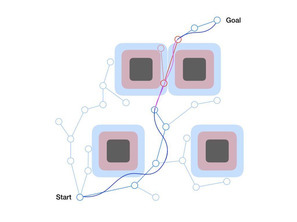
Figure 7. By considering two different planners, each with a different tracking error bound, our algorithm is able to find a guaranteed safe “meta-plan” that prefers the less precise but faster-moving blue planner but reverts to the more precise but slower red planner in the vicinity of obstacles. This leads to natural, intuitive behavior that optimally trades off planner conservatism with vehicle maneuvering speed.

Safe Switching

The key to making this work is to ensure that all transitions between planners are safe. This can get a little complicated, but the main idea is that a transition between two planners — call them A and B — is safe if we can guarantee that the invariant set computed for A is contained within that for B. For many pairs of planners this is true, e.g. switching from the blue bound to the red bound in Fig. 7. But often it is not. In general, we need to solve a dynamic game very similar to the original one in FaSTrack, but where we want to know the set of states that we will never leave and from which we can guarantee we end up inside B’s invariant set. Usually, the resulting safe switching bound (SSB) is slightly larger than A’s tracking error bound (TEB), as shown below.

Figure 8. The safe switching bound for a transition between a planner with a large tracking error bound to one with a small tracking error bound is generally larger than the large tracking error bound, as shown.

Efficient Online Meta-Planning

To do this efficiently in real time, we use a modified version of the classical RRT algorithm. Usually, RRTs work by sampling points in state space and connecting them with line segments to form a tree rooted at the start point. In our case, we replace the line segments with the actual trajectories generated by individual planners. In order to find the shortest route to the goal, we favor planners that can move more quickly, trying them first and only resorting to slower-moving planners if the faster ones fail.

We do have to be careful to ensure safe switching bounds are satisfied, however. This is especially important in cases where the meta-planner decides to transition to a more precise, slower-moving planner, as in the example above. In such cases, we implement a one-step virtual backtracking algorithm in which we make sure the preceding trajectory segment is collision-free using the switching controller.

Implementation

We implemented both FaSTrack and Meta-Planning in C++ / ROS, using low-level motion planners from the Open Motion Planning Library (OMPL). Simulated results are shown below, with (right) and without (left) our optimal controller. As you can see, simply using a linear feedback (LQR) controller (left) provides no guarantees about staying inside the tracking error bound.

Figures 9 & 10. (Left) A standard LQR controller is unable to keep the quadrotor within the tracking error bound. (Right) The optimal tracking controller keeps the quadrotor within the tracking bound, even during radical changes in the planned trajectory.

It also works on hardware! We tested on the open-source Crazyflie 2.0 quadrotor platform. As you can see in Fig. 12, we manage to stay inside the tracking bound at all times, even when switching planners.

Figures 11 & 12. (Left) A Crazyflie 2.0 quadrotor being observed by an OptiTrack motion capture system. (Right) Position traces from a hardware test of the meta planning algorithm. As shown, the tracking system stays within the tracking error bound at all times, even during the planner switch that occurs approximately 4.5 seconds after the start.

This article was initially published on the BAIR blog, and appears here with the authors’ permission.

This post is based on the following papers:

• FaSTrack: a Modular Framework for Fast and Guaranteed Safe Motion Planning
  Sylvia Herbert*, Mo Chen*, SooJean Han, Somil Bansal, Jaime F. Fisac, and Claire J. Tomlin
  Paper, Website

• Planning, Fast and Slow: A Framework for Adaptive Real-Time Safe Trajectory Planning
  David Fridovich-Keil*, Sylvia Herbert*, Jaime F. Fisac*, Sampada Deglurkar, and Claire J. Tomlin
  Paper, Github (code to appear soon)

We would like to thank our coauthors; developing FaSTrack has been a team effort and we are incredibly fortunate to have a fantastic set of colleagues on this project.