By Andre He, Vivek Myers

A longstanding goal of the field of robot learning has been to create generalist agents that can perform tasks for humans. Natural language has the potential to be an easy-to-use interface for humans to specify arbitrary tasks, but it is difficult to train robots to follow language instructions. Approaches like language-conditioned behavioral cloning (LCBC) train policies to directly imitate expert actions conditioned on language, but require humans to annotate all training trajectories and generalize poorly across scenes and behaviors. Meanwhile, recent goal-conditioned approaches perform much better at general manipulation tasks, but do not enable easy task specification for human operators. How can we reconcile the ease of specifying tasks through LCBC-like approaches with the performance improvements of goal-conditioned learning?

Conceptually, an instruction-following robot requires two capabilities. It needs to ground the language instruction in the physical environment, and then be able to carry out a sequence of actions to complete the intended task. These capabilities do not need to be learned end-to-end from human-annotated trajectories alone, but can instead be learned separately from the appropriate data sources. Vision-language data from non-robot sources can help learn language grounding with generalization to diverse instructions and visual scenes. Meanwhile, unlabeled robot trajectories can be used to train a robot to reach specific goal states, even when they are not associated with language instructions.

Conditioning on visual goals (i.e. goal images) provides complementary benefits for policy learning. As a form of task specification, goals are desirable for scaling because they can be freely generated hindsight relabeling (any state reached along a trajectory can be a goal). This allows policies to be trained via goal-conditioned behavioral cloning (GCBC) on large amounts of unannotated and unstructured trajectory data, including data collected autonomously by the robot itself. Goals are also easier to ground since, as images, they can be directly compared pixel-by-pixel with other states.

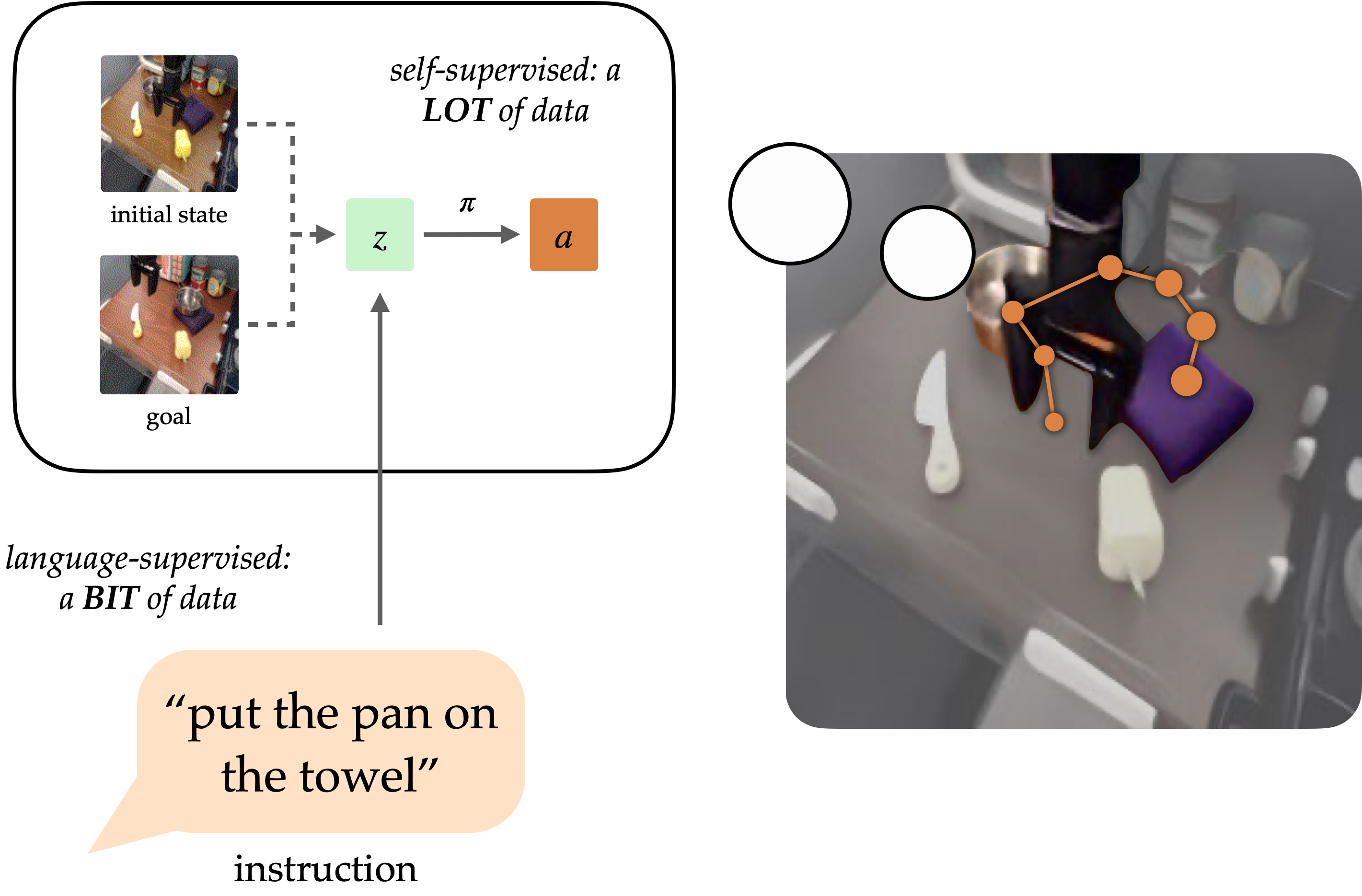
However, goals are less intuitive for human users than natural language. In most cases, it is easier for a user to describe the task they want performed than it is to provide a goal image, which would likely require performing the task anyways to generate the image. By exposing a language interface for goal-conditioned policies, we can combine the strengths of both goal- and language- task specification to enable generalist robots that can be easily commanded. Our method, discussed below, exposes such an interface to generalize to diverse instructions and scenes using vision-language data, and improve its physical skills by digesting large unstructured robot datasets.

Goal representations for instruction following

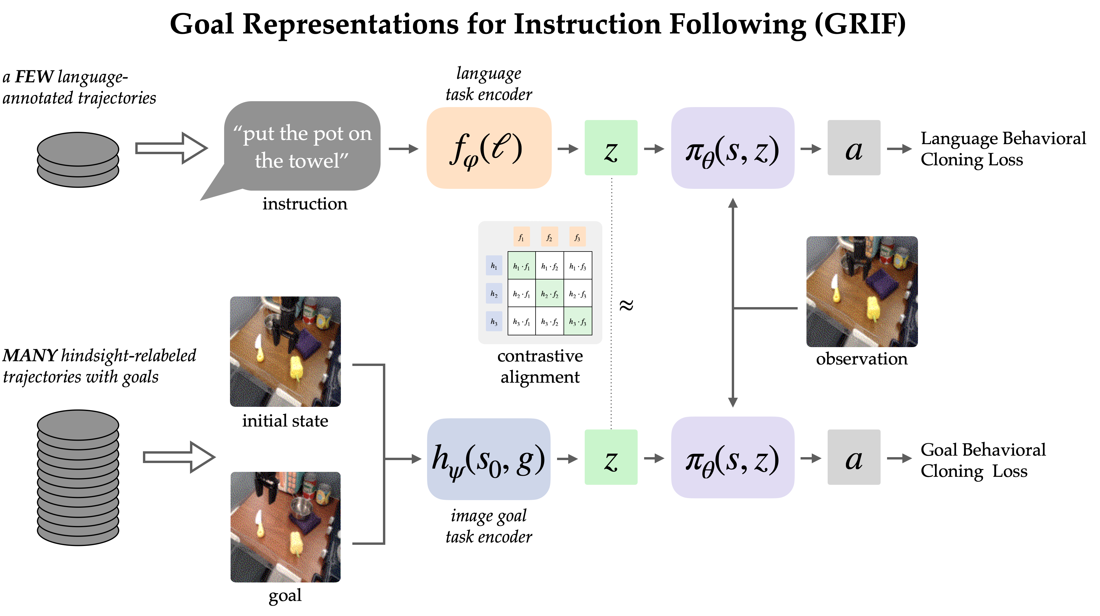
The GRIF model consists of a language encoder, a goal encoder, and a policy network. The encoders respectively map language instructions and goal images into a shared task representation space, which conditions the policy network when predicting actions. The model can effectively be conditioned on either language instructions or goal images to predict actions, but we are primarily using goal-conditioned training as a way to improve the language-conditioned use case.

Our approach, Goal Representations for Instruction Following (GRIF), jointly trains a language- and a goal- conditioned policy with aligned task representations. Our key insight is that these representations, aligned across language and goal modalities, enable us to effectively combine the benefits of goal-conditioned learning with a language-conditioned policy. The learned policies are then able to generalize across language and scenes after training on mostly unlabeled demonstration data.

We trained GRIF on a version of the Bridge-v2 dataset containing 7k labeled demonstration trajectories and 47k unlabeled ones within a kitchen manipulation setting. Since all the trajectories in this dataset had to be manually annotated by humans, being able to directly use the 47k trajectories without annotation significantly improves efficiency.

To learn from both types of data, GRIF is trained jointly with language-conditioned behavioral cloning (LCBC) and goal-conditioned behavioral cloning (GCBC). The labeled dataset contains both language and goal task specifications, so we use it to supervise both the language- and goal-conditioned predictions (i.e. LCBC and GCBC). The unlabeled dataset contains only goals and is used for GCBC. The difference between LCBC and GCBC is just a matter of selecting the task representation from the corresponding encoder, which is passed into a shared policy network to predict actions.

By sharing the policy network, we can expect some improvement from using the unlabeled dataset for goal-conditioned training. However,GRIF enables much stronger transfer between the two modalities by recognizing that some language instructions and goal images specify the same behavior. In particular, we exploit this structure by requiring that language- and goal- representations be similar for the same semantic task. Assuming this structure holds, unlabeled data can also benefit the language-conditioned policy since the goal representation approximates that of the missing instruction.

Alignment through contrastive learning

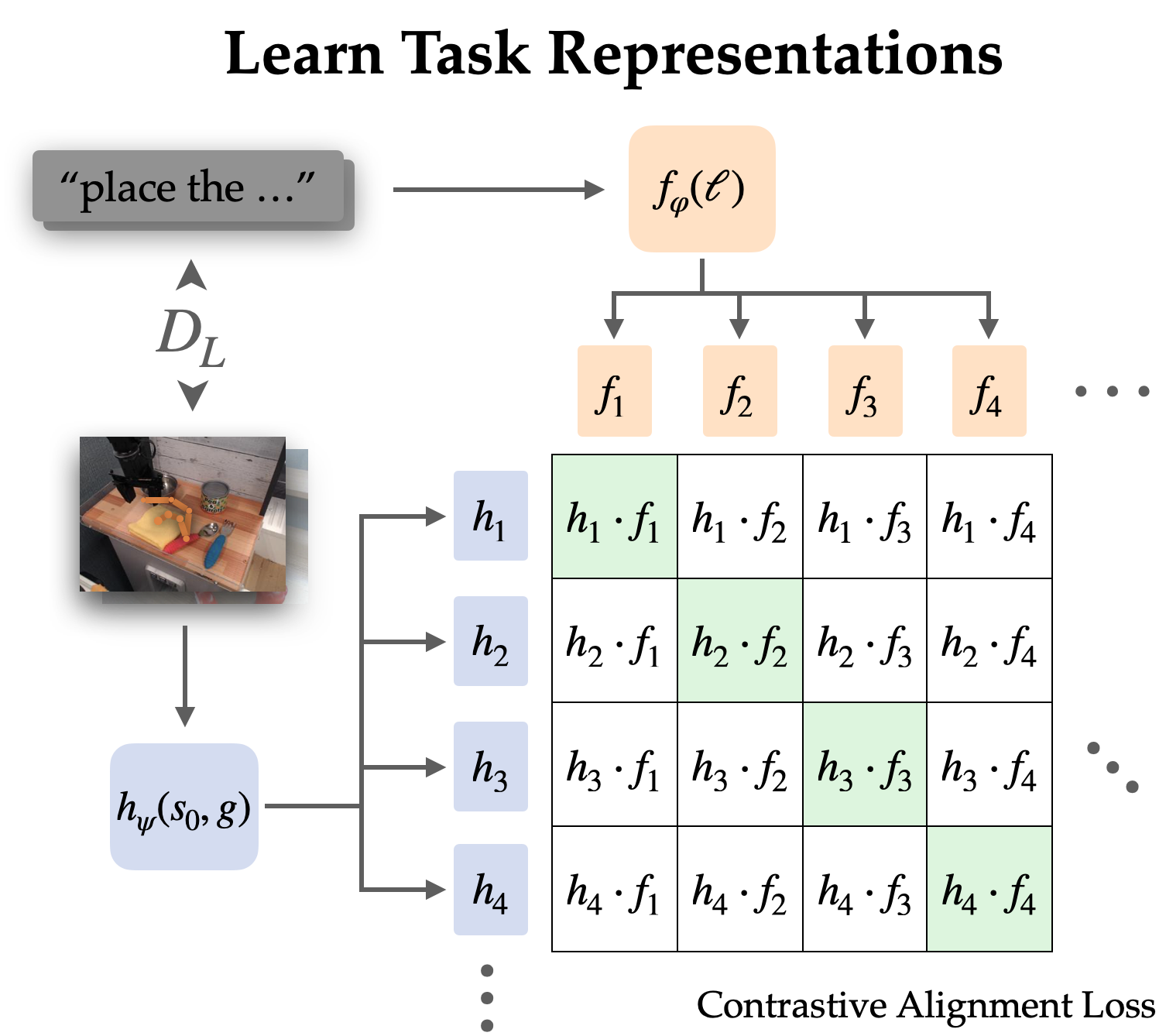
We explicitly align representations between goal-conditioned and language-conditioned tasks on the labeled dataset through contrastive learning.

Since language often describes relative change, we choose to align representations of state-goal pairs with the language instruction (as opposed to just goal with language). Empirically, this also makes the representations easier to learn since they can omit most information in the images and focus on the change from state to goal.

We learn this alignment structure through an infoNCE objective on instructions and images from the labeled dataset. We train dual image and text encoders by doing contrastive learning on matching pairs of language and goal representations. The objective encourages high similarity between representations of the same task and low similarity for others, where the negative examples are sampled from other trajectories.

When using naive negative sampling (uniform from the rest of the dataset), the learned representations often ignored the actual task and simply aligned instructions and goals that referred to the same scenes. To use the policy in the real world, it is not very useful to associate language with a scene; rather we need it to disambiguate between different tasks in the same scene. Thus, we use a hard negative sampling strategy, where up to half the negatives are sampled from different trajectories in the same scene.

Naturally, this contrastive learning setup teases at pre-trained vision-language models like CLIP. They demonstrate effective zero-shot and few-shot generalization capability for vision-language tasks, and offer a way to incorporate knowledge from internet-scale pre-training. However, most vision-language models are designed for aligning a single static image with its caption without the ability to understand changes in the environment, and they perform poorly when having to pay attention to a single object in cluttered scenes.

To address these issues, we devise a mechanism to accommodate and fine-tune CLIP for aligning task representations. We modify the CLIP architecture so that it can operate on a pair of images combined with early fusion (stacked channel-wise). This turns out to be a capable initialization for encoding pairs of state and goal images, and one which is particularly good at preserving the pre-training benefits from CLIP.

Robot policy results

For our main result, we evaluate the GRIF policy in the real world on 15 tasks across 3 scenes. The instructions are chosen to be a mix of ones that are well-represented in the training data and novel ones that require some degree of compositional generalization. One of the scenes also features an unseen combination of objects.

We compare GRIF against plain LCBC and stronger baselines inspired by prior work like LangLfP and BC-Z. LLfP corresponds to jointly training with LCBC and GCBC. BC-Z is an adaptation of the namesake method to our setting, where we train on LCBC, GCBC, and a simple alignment term. It optimizes the cosine distance loss between the task representations and does not use image-language pre-training.

The policies were susceptible to two main failure modes. They can fail to understand the language instruction, which results in them attempting another task or performing no useful actions at all. When language grounding is not robust, policies might even start an unintended task after having done the right task, since the original instruction is out of context.

Examples of grounding failures

“put the mushroom in the metal pot”

“put the spoon on the towel”

“put the yellow bell pepper on the cloth”

“put the yellow bell pepper on the cloth”

The other failure mode is failing to manipulate objects. This can be due to missing a grasp, moving imprecisely, or releasing objects at the incorrect time. We note that these are not inherent shortcomings of the robot setup, as a GCBC policy trained on the entire dataset can consistently succeed in manipulation. Rather, this failure mode generally indicates an ineffectiveness in leveraging goal-conditioned data.

Examples of manipulation failures

“move the bell pepper to the left of the table”

“put the bell pepper in the pan”

“move the towel next to the microwave”

Comparing the baselines, they each suffered from these two failure modes to different extents. LCBC relies solely on the small labeled trajectory dataset, and its poor manipulation capability prevents it from completing any tasks. LLfP jointly trains the policy on labeled and unlabeled data and shows significantly improved manipulation capability from LCBC. It achieves reasonable success rates for common instructions, but fails to ground more complex instructions. BC-Z’s alignment strategy also improves manipulation capability, likely because alignment improves the transfer between modalities. However, without external vision-language data sources, it still struggles to generalize to new instructions.

GRIF shows the best generalization while also having strong manipulation capabilities. It is able to ground the language instructions and carry out the task even when many distinct tasks are possible in the scene. We show some rollouts and the corresponding instructions below.

Policy Rollouts from GRIF

“move the pan to the front”

“put the bell pepper in the pan”

“put the knife on the purple cloth”

“put the spoon on the towel”

Conclusion

GRIF enables a robot to utilize large amounts of unlabeled trajectory data to learn goal-conditioned policies, while providing a “language interface” to these policies via aligned language-goal task representations. In contrast to prior language-image alignment methods, our representations align changes in state to language, which we show leads to significant improvements over standard CLIP-style image-language alignment objectives. Our experiments demonstrate that our approach can effectively leverage unlabeled robotic trajectories, with large improvements in performance over baselines and methods that only use the language-annotated data

Our method has a number of limitations that could be addressed in future work. GRIF is not well-suited for tasks where instructions say more about how to do the task than what to do (e.g., “pour the water slowly”)—such qualitative instructions might require other types of alignment losses that consider the intermediate steps of task execution. GRIF also assumes that all language grounding comes from the portion of our dataset that is fully annotated or a pre-trained VLM. An exciting direction for future work would be to extend our alignment loss to utilize human video data to learn rich semantics from Internet-scale data. Such an approach could then use this data to improve grounding on language outside the robot dataset and enable broadly generalizable robot policies that can follow user instructions.

This post is based on the following paper:

• Goal Representations for Instruction Following: A Semi-Supervised Language Interface to Control
  Vivek Myers*, Andre He*, Kuan Fang, Homer Walke, Philippe Hansen-Estruch, Ching-An Cheng, Mihai Jalobeanu, Andrey Kolobov, Anca Dragan, and Sergey Levine

Commercial and industrial deployments of robot fleets: package delivery (top left), food delivery (bottom left), e-commerce order fulfillment at Ambi Robotics (top right), autonomous taxis at Waymo (bottom right).

In the last few years we have seen an exciting development in robotics and artificial intelligence: large fleets of robots have left the lab and entered the real world. Waymo, for example, has over 700 self-driving cars operating in Phoenix and San Francisco and is currently expanding to Los Angeles. Other industrial deployments of robot fleets include applications like e-commerce order fulfillment at Amazon and Ambi Robotics as well as food delivery at Nuro and Kiwibot.

Figure 1: “Interactive Fleet Learning” (IFL) refers to robot fleets in industry and academia that fall back on human teleoperators when necessary and continually learn from them over time.

These robots use recent advances in deep learning to operate autonomously in unstructured environments. By pooling data from all robots in the fleet, the entire fleet can efficiently learn from the experience of each individual robot. Furthermore, due to advances in cloud robotics, the fleet can offload data, memory, and computation (e.g., training of large models) to the cloud via the Internet. This approach is known as “Fleet Learning,” a term popularized by Elon Musk in 2016 press releases about Tesla Autopilot and used in press communications by Toyota Research Institute, Wayve AI, and others. A robot fleet is a modern analogue of a fleet of ships, where the word fleet has an etymology tracing back to flēot (‘ship’) and flēotan (‘float’) in Old English.

Data-driven approaches like fleet learning, however, face the problem of the “long tail”: the robots inevitably encounter new scenarios and edge cases that are not represented in the dataset. Naturally, we can’t expect the future to be the same as the past! How, then, can these robotics companies ensure sufficient reliability for their services?

One answer is to fall back on remote humans over the Internet, who can interactively take control and “tele-operate” the system when the robot policy is unreliable during task execution. Teleoperation has a rich history in robotics: the world’s first robots were teleoperated during WWII to handle radioactive materials, and the Telegarden pioneered robot control over the Internet in 1994. With continual learning, the human teleoperation data from these interventions can iteratively improve the robot policy and reduce the robots’ reliance on their human supervisors over time. Rather than a discrete jump to full robot autonomy, this strategy offers a continuous alternative that approaches full autonomy over time while simultaneously enabling reliability in robot systems today.

The use of human teleoperation as a fallback mechanism is increasingly popular in modern robotics companies: Waymo calls it “fleet response,” Zoox calls it “TeleGuidance,” and Amazon calls it “continual learning.” Last year, a software platform for remote driving called Phantom Auto was recognized by Time Magazine as one of their Top 10 Inventions of 2022. And just last month, John Deere acquired SparkAI, a startup that develops software for resolving edge cases with humans in the loop.

A remote human teleoperator at Phantom Auto, a software platform for enabling remote driving over the Internet.

Despite this growing trend in industry, however, there has been comparatively little focus on this topic in academia. As a result, robotics companies have had to rely on ad hoc solutions for determining when their robots should cede control. The closest analogue in academia is interactive imitation learning (IIL), a paradigm in which a robot intermittently cedes control to a human supervisor and learns from these interventions over time. There have been a number of IIL algorithms in recent years for the single-robot, single-human setting including DAgger and variants such as HG-DAgger, SafeDAgger, EnsembleDAgger, and ThriftyDAgger; nevertheless, when and how to switch between robot and human control is still an open problem. This is even less understood when the notion is generalized to robot fleets, with multiple robots and multiple human supervisors.

IFL Formalism and Algorithms

To this end, in a recent paper at the Conference on Robot Learning we introduced the paradigm of Interactive Fleet Learning (IFL), the first formalism in the literature for interactive learning with multiple robots and multiple humans. As we’ve seen that this phenomenon already occurs in industry, we can now use the phrase “interactive fleet learning” as unified terminology for robot fleet learning that falls back on human control, rather than keep track of the names of every individual corporate solution (“fleet response”, “TeleGuidance”, etc.). IFL scales up robot learning with four key components:

1. On-demand supervision. Since humans cannot effectively monitor the execution of multiple robots at once and are prone to fatigue, the allocation of robots to humans in IFL is automated by some allocation policy . Supervision is requested “on-demand” by the robots rather than placing the burden of continuous monitoring on the humans.
2. Fleet supervision. On-demand supervision enables effective allocation of limited human attention to large robot fleets. IFL allows the number of robots to significantly exceed the number of humans (e.g., by a factor of 10:1 or more).
3. Continual learning. Each robot in the fleet can learn from its own mistakes as well as the mistakes of the other robots, allowing the amount of required human supervision to taper off over time.
4. The Internet. Thanks to mature and ever-improving Internet technology, the human supervisors do not need to be physically present. Modern computer networks enable real-time remote teleoperation at vast distances.

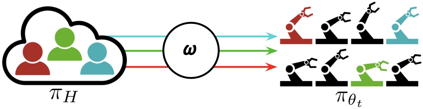
In the Interactive Fleet Learning (IFL) paradigm, M humans are allocated to the robots that need the most help in a fleet of N robots (where N can be much larger than M). The robots share policy and learn from human interventions over time.

We assume that the robots share a common control policy and that the humans share a common control policy . We also assume that the robots operate in independent environments with identical state and action spaces (but not identical states). Unlike a robot swarm of typically low-cost robots that coordinate to achieve a common objective in a shared environment, a robot fleet simultaneously executes a shared policy in distinct parallel environments (e.g., different bins on an assembly line).

The goal in IFL is to find an optimal supervisor allocation policy , a mapping from (the state of all robots at time t) and the shared policy to a binary matrix that indicates which human will be assigned to which robot at time t. The IFL objective is a novel metric we call the “return on human effort” (ROHE):

where the numerator is the total reward across robots and timesteps and the denominator is the total amount of human actions across robots and timesteps. Intuitively, the ROHE measures the performance of the fleet normalized by the total human supervision required. See the paper for more of the mathematical details.

Using this formalism, we can now instantiate and compare IFL algorithms (i.e., allocation policies) in a principled way. We propose a family of IFL algorithms called Fleet-DAgger, where the policy learning algorithm is interactive imitation learning and each Fleet-DAgger algorithm is parameterized by a unique priority function that each robot in the fleet uses to assign itself a priority score. Similar to scheduling theory, higher priority robots are more likely to receive human attention. Fleet-DAgger is general enough to model a wide range of IFL algorithms, including IFL adaptations of existing single-robot, single-human IIL algorithms such as EnsembleDAgger and ThriftyDAgger. Note, however, that the IFL formalism isn’t limited to Fleet-DAgger: policy learning could be performed with a reinforcement learning algorithm like PPO, for instance.

IFL Benchmark and Experiments

To determine how to best allocate limited human attention to large robot fleets, we need to be able to empirically evaluate and compare different IFL algorithms. To this end, we introduce the IFL Benchmark, an open-source Python toolkit available on Github to facilitate the development and standardized evaluation of new IFL algorithms. We extend NVIDIA Isaac Gym, a highly optimized software library for end-to-end GPU-accelerated robot learning released in 2021, without which the simulation of hundreds or thousands of learning robots would be computationally intractable. Using the IFL Benchmark, we run large-scale simulation experiments with N = 100 robots, M = 10 algorithmic humans, 5 IFL algorithms, and 3 high-dimensional continuous control environments (Figure 1, left).

We also evaluate IFL algorithms in a real-world image-based block pushing task with N = 4 robot arms and M = 2 remote human teleoperators (Figure 1, right). The 4 arms belong to 2 bimanual ABB YuMi robots operating simultaneously in 2 separate labs about 1 kilometer apart, and remote humans in a third physical location perform teleoperation through a keyboard interface when requested. Each robot pushes a cube toward a unique goal position randomly sampled in the workspace; the goals are programmatically generated in the robots’ overhead image observations and automatically resampled when the previous goals are reached. Physical experiment results suggest trends that are approximately consistent with those observed in the benchmark environments.

Takeaways and Future Directions

To address the gap between the theory and practice of robot fleet learning as well as facilitate future research, we introduce new formalisms, algorithms, and benchmarks for Interactive Fleet Learning. Since IFL does not dictate a specific form or architecture for the shared robot control policy, it can be flexibly synthesized with other promising research directions. For instance, diffusion policies, recently demonstrated to gracefully handle multimodal data, can be used in IFL to allow heterogeneous human supervisor policies. Alternatively, multi-task language-conditioned Transformers like RT-1 and PerAct can be effective “data sponges” that enable the robots in the fleet to perform heterogeneous tasks despite sharing a single policy. The systems aspect of IFL is another compelling research direction: recent developments in cloud and fog robotics enable robot fleets to offload all supervisor allocation, model training, and crowdsourced teleoperation to centralized servers in the cloud with minimal network latency.

While Moravec’s Paradox has so far prevented robotics and embodied AI from fully enjoying the recent spectacular success that Large Language Models (LLMs) like GPT-4 have demonstrated, the “bitter lesson” of LLMs is that supervised learning at unprecedented scale is what ultimately leads to the emergent properties we observe. Since we don’t yet have a supply of robot control data nearly as plentiful as all the text and image data on the Internet, the IFL paradigm offers one path forward for scaling up supervised robot learning and deploying robot fleets reliably in today’s world.

This post is based on the paper “Fleet-DAgger: Interactive Robot Fleet Learning with Scalable Human Supervision” by Ryan Hoque, Lawrence Chen, Satvik Sharma, Karthik Dharmarajan, Brijen Thananjeyan, Pieter Abbeel, and Ken Goldberg, presented at the Conference on Robot Learning (CoRL) 2022. For more details, see the paper on arXiv, CoRL presentation video on YouTube, open-source codebase on Github, high-level summary on Twitter, and project website.

If you would like to cite this article, please use the following bibtex:

@article{ifl_blog,
    title={Interactive Fleet Learning},
    author={Hoque, Ryan},
    url={https://bair.berkeley.edu/blog/2023/04/06/ifl/},
    journal={Berkeley Artificial Intelligence Research Blog},
    year={2023} 
}

By Jędrzej Orbik, Charles Sun, Coline Devin, Glen Berseth

Reinforcement learning provides a conceptual framework for autonomous agents to learn from experience, analogously to how one might train a pet with treats. But practical applications of reinforcement learning are often far from natural: instead of using RL to learn through trial and error by actually attempting the desired task, typical RL applications use a separate (usually simulated) training phase. For example, AlphaGo did not learn to play Go by competing against thousands of humans, but rather by playing against itself in simulation. While this kind of simulated training is appealing for games where the rules are perfectly known, applying this to real world domains such as robotics can require a range of complex approaches, such as the use of simulated data, or instrumenting real-world environments in various ways to make training feasible under laboratory conditions. Can we instead devise reinforcement learning systems for robots that allow them to learn directly “on-the-job”, while performing the task that they are required to do? In this blog post, we will discuss ReLMM, a system that we developed that learns to clean up a room directly with a real robot via continual learning.

We evaluate our method on different tasks that range in difficulty. The top-left task has uniform white blobs to pickup with no obstacles, while other rooms have objects of diverse shapes and colors, obstacles that increase navigation difficulty and obscure the objects and patterned rugs that make it difficult to see the objects against the ground.

To enable “on-the-job” training in the real world, the difficulty of collecting more experience is prohibitive. If we can make training in the real world easier, by making the data gathering process more autonomous without requiring human monitoring or intervention, we can further benefit from the simplicity of agents that learn from experience. In this work, we design an “on-the-job” mobile robot training system for cleaning by learning to grasp objects throughout different rooms.

Lesson 1: The Benefits of Modular Policies for Robots.

People are not born one day and performing job interviews the next. There are many levels of tasks people learn before they apply for a job as we start with the easier ones and build on them. In ReLMM, we make use of this concept by allowing robots to train common-reusable skills, such as grasping, by first encouraging the robot to prioritize training these skills before learning later skills, such as navigation. Learning in this fashion has two advantages for robotics. The first advantage is that when an agent focuses on learning a skill, it is more efficient at collecting data around the local state distribution for that skill.

That is shown in the figure above, where we evaluated the amount of prioritized grasping experience needed to result in efficient mobile manipulation training. The second advantage to a multi-level learning approach is that we can inspect the models trained for different tasks and ask them questions, such as, “can you grasp anything right now” which is helpful for navigation training that we describe next.

Training this multi-level policy was not only more efficient than learning both skills at the same time but it allowed for the grasping controller to inform the navigation policy. Having a model that estimates the uncertainty in its grasp success (Ours above) can be used to improve navigation exploration by skipping areas without graspable objects, in contrast to No Uncertainty Bonus which does not use this information. The model can also be used to relabel data during training so that in the unlucky case when the grasping model was unsuccessful trying to grasp an object within its reach, the grasping policy can still provide some signal by indicating that an object was there but the grasping policy has not yet learned how to grasp it. Moreover, learning modular models has engineering benefits. Modular training allows for reusing skills that are easier to learn and can enable building intelligent systems one piece at a time. This is beneficial for many reasons, including safety evaluation and understanding.

Lesson 2: Learning systems beat hand-coded systems, given time

Many robotics tasks that we see today can be solved to varying levels of success using hand-engineered controllers. For our room cleaning task, we designed a hand-engineered controller that locates objects using image clustering and turns towards the nearest detected object at each step. This expertly designed controller performs very well on the visually salient balled socks and takes reasonable paths around the obstacles but it can not learn an optimal path to collect the objects quickly, and it struggles with visually diverse rooms. As shown in video 3 below, the scripted policy gets distracted by the white patterned carpet while trying to locate more white objects to grasp.

1)
2)
3)
4)
We show a comparison between (1) our policy at the beginning of training (2) our policy at the end of training (3) the scripted policy. In (4) we can see the robot’s performance improve over time, and eventually exceed the scripted policy at quickly collecting the objects in the room.

Given we can use experts to code this hand-engineered controller, what is the purpose of learning? An important limitation of hand-engineered controllers is that they are tuned for a particular task, for example, grasping white objects. When diverse objects are introduced, which differ in color and shape, the original tuning may no longer be optimal. Rather than requiring further hand-engineering, our learning-based method is able to adapt itself to various tasks by collecting its own experience.

However, the most important lesson is that even if the hand-engineered controller is capable, the learning agent eventually surpasses it given enough time. This learning process is itself autonomous and takes place while the robot is performing its job, making it comparatively inexpensive. This shows the capability of learning agents, which can also be thought of as working out a general way to perform an “expert manual tuning” process for any kind of task. Learning systems have the ability to create the entire control algorithm for the robot, and are not limited to tuning a few parameters in a script. The key step in this work allows these real-world learning systems to autonomously collect the data needed to enable the success of learning methods.

This post is based on the paper “Fully Autonomous Real-World Reinforcement Learning with Applications to Mobile Manipulation”, presented at CoRL 2021. You can find more details in our paper, on our website and the on the video. We provide code to reproduce our experiments. We thank Sergey Levine for his valuable feedback on this blog post.

In cooperative multi-agent reinforcement learning (MARL), due to its on-policy nature, policy gradient (PG) methods are typically believed to be less sample efficient than value decomposition (VD) methods, which are off-policy. However, some recent empirical studies demonstrate that with proper input representation and hyper-parameter tuning, multi-agent PG can achieve surprisingly strong performance compared to off-policy VD methods.

Why could PG methods work so well? In this post, we will present concrete analysis to show that in certain scenarios, e.g., environments with a highly multi-modal reward landscape, VD can be problematic and lead to undesired outcomes. By contrast, PG methods with individual policies can converge to an optimal policy in these cases. In addition, PG methods with auto-regressive (AR) policies can learn multi-modal policies.

Figure 1: different policy representation for the 4-player permutation game.

CTDE in Cooperative MARL: VD and PG methods

Centralized training and decentralized execution (CTDE) is a popular framework in cooperative MARL. It leverages global information for more effective training while keeping the representation of individual policies for testing. CTDE can be implemented via value decomposition (VD) or policy gradient (PG), leading to two different types of algorithms.

VD methods learn local Q networks and a mixing function that mixes the local Q networks to a global Q function. The mixing function is usually enforced to satisfy the Individual-Global-Max (IGM) principle, which guarantees the optimal joint action can be computed by greedily choosing the optimal action locally for each agent.

By contrast, PG methods directly apply policy gradient to learn an individual policy and a centralized value function for each agent. The value function takes as its input the global state (e.g., MAPPO) or the concatenation of all the local observations (e.g., MADDPG), for an accurate global value estimate.

The permutation game: a simple counterexample where VD fails

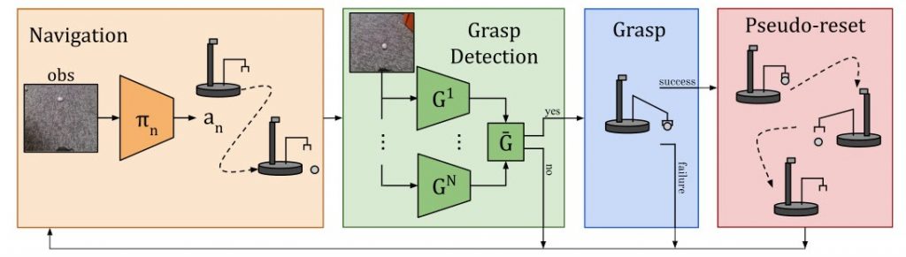
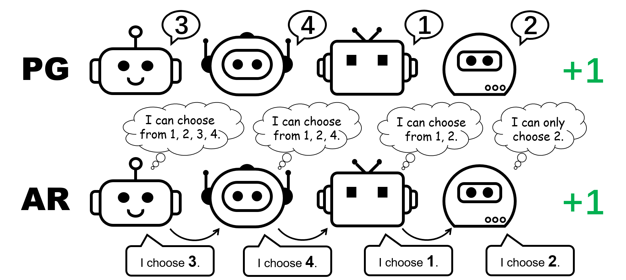
We start our analysis by considering a stateless cooperative game, namely the permutation game. In an -player permutation game, each agent can output actions . Agents receive reward if their actions are mutually different, i.e., the joint action is a permutation over ; otherwise, they receive reward. Note that there are symmetric optimal strategies in this game.

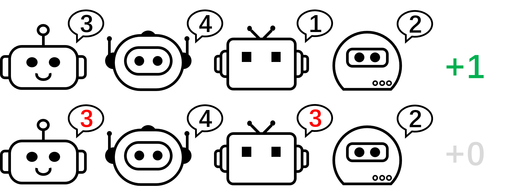
Figure 2: the 4-player permutation game.

Let us focus on the 2-player permutation game for our discussion. In this setting, if we apply VD to the game, the global Q-value will factorize to

where and are local Q-functions, is the global Q-function, and is the mixing function that, as required by VD methods, satisfies the IGM principle.

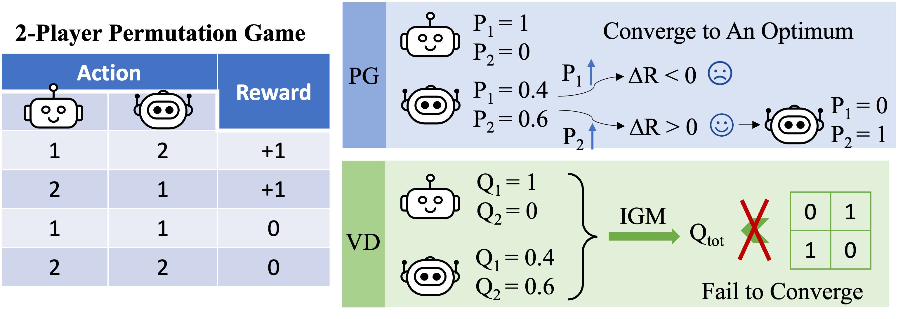
Figure 3: high-level intuition on why VD fails in the 2-player permutation game.

We formally prove that VD cannot represent the payoff of the 2-player permutation game by contradiction. If VD methods were able to represent the payoff, we would have

However, if either of these two agents have different local Q values, e.g. , then according to the IGM principle, we must have

Otherwise, if and , then

As a result, value decomposition cannot represent the payoff matrix of the 2-player permutation game.

What about PG methods? Individual policies can indeed represent an optimal policy for the permutation game. Moreover, stochastic gradient descent can guarantee PG to converge to one of these optima under mild assumptions. This suggests that, even though PG methods are less popular in MARL compared with VD methods, they can be preferable in certain cases that are common in real-world applications, e.g., games with multiple strategy modalities.

We also remark that in the permutation game, in order to represent an optimal joint policy, each agent must choose distinct actions. Consequently, a successful implementation of PG must ensure that the policies are agent-specific. This can be done by using either individual policies with unshared parameters (referred to as PG-Ind in our paper), or an agent-ID conditioned policy (PG-ID).

PG outperform best VD methods on popular MARL testbeds

Going beyond the simple illustrative example of the permutation game, we extend our study to popular and more realistic MARL benchmarks. In addition to StarCraft Multi-Agent Challenge (SMAC), where the effectiveness of PG and agent-conditioned policy input has been verified, we show new results in Google Research Football (GRF) and multi-player Hanabi Challenge.

Figure 4: (top) winning rates of PG methods on GRF; (bottom) best and average evaluation scores on Hanabi-Full.

In GRF, PG methods outperform the state-of-the-art VD baseline (CDS) in 5 scenarios. Interestingly, we also notice that individual policies (PG-Ind) without parameter sharing achieve comparable, sometimes even higher winning rates, compared to agent-specific policies (PG-ID) in all 5 scenarios. We evaluate PG-ID in the full-scale Hanabi game with varying numbers of players (2-5 players) and compare them to SAD, a strong off-policy Q-learning variant in Hanabi, and Value Decomposition Networks (VDN). As demonstrated in the above table, PG-ID is able to produce results comparable to or better than the best and average rewards achieved by SAD and VDN with varying numbers of players using the same number of environment steps.

Beyond higher rewards: learning multi-modal behavior via auto-regressive policy modeling

Besides learning higher rewards, we also study how to learn multi-modal policies in cooperative MARL. Let’s go back to the permutation game. Although we have proved that PG can effectively learn an optimal policy, the strategy mode that it finally reaches can highly depend on the policy initialization. Thus, a natural question will be:

Can we learn a single policy that can cover all the optimal modes?

In the decentralized PG formulation, the factorized representation of a joint policy can only represent one particular mode. Therefore, we propose an enhanced way to parameterize the policies for stronger expressiveness — the auto-regressive (AR) policies.

Figure 5: comparison between individual policies (PG) and auto-regressive policies (AR) in the 4-player permutation game.

Formally, we factorize the joint policy of agents into the form of

where the action produced by agent depends on its own observation and all the actions from previous agents . The auto-regressive factorization can represent any joint policy in a centralized MDP. The only modification to each agent’s policy is the input dimension, which is slightly enlarged by including previous actions; and the output dimension of each agent’s policy remains unchanged.

With such a minimal parameterization overhead, AR policy substantially improves the representation power of PG methods. We remark that PG with AR policy (PG-AR) can simultaneously represent all optimal policy modes in the permutation game.

Figure: the heatmaps of actions for policies learned by PG-Ind (left) and PG-AR (middle), and the heatmap for rewards (right); while PG-Ind only converge to a specific mode in the 4-player permutation game, PG-AR successfully discovers all the optimal modes.

In more complex environments, including SMAC and GRF, PG-AR can learn interesting emergent behaviors that require strong intra-agent coordination that may never be learned by PG-Ind.

Figure 6: (top) emergent behavior induced by PG-AR in SMAC and GRF. On the 2m_vs_1z map of SMAC, the marines keep standing and attack alternately while ensuring there is only one attacking marine at each timestep; (bottom) in the academy_3_vs_1_with_keeper scenario of GRF, agents learn a “Tiki-Taka” style behavior: each player keeps passing the ball to their teammates.

Discussions and Takeaways

In this post, we provide a concrete analysis of VD and PG methods in cooperative MARL. First, we reveal the limitation on the expressiveness of popular VD methods, showing that they could not represent optimal policies even in a simple permutation game. By contrast, we show that PG methods are provably more expressive. We empirically verify the expressiveness advantage of PG on popular MARL testbeds, including SMAC, GRF, and Hanabi Challenge. We hope the insights from this work could benefit the community towards more general and more powerful cooperative MARL algorithms in the future.

This post is based on our paper in joint with Zelai Xu: Revisiting Some Common Practices in Cooperative Multi-Agent Reinforcement Learning (paper, website).

By Nathan Lambert, Aaron Snoswell, Sarah Dean, Thomas Krendl Gilbert, and Tom Zick

Deep reinforcement learning (DRL) is transitioning from a research field focused on game playing to a technology with real-world applications. Notable examples include DeepMind’s work on controlling a nuclear reactor or on improving Youtube video compression, or Tesla attempting to use a method inspired by MuZero for autonomous vehicle behavior planning. But the exciting potential for real world applications of RL should also come with a healthy dose of caution – for example RL policies are well known to be vulnerable to exploitation, and methods for safe and robust policy development are an active area of research.

At the same time as the emergence of powerful RL systems in the real world, the public and researchers are expressing an increased appetite for fair, aligned, and safe machine learning systems. The focus of these research efforts to date has been to account for shortcomings of datasets or supervised learning practices that can harm individuals. However the unique ability of RL systems to leverage temporal feedback in learning complicates the types of risks and safety concerns that can arise.

This post expands on our recent whitepaper and research paper, where we aim to illustrate the different modalities harms can take when augmented with the temporal axis of RL. To combat these novel societal risks, we also propose a new kind of documentation for dynamic Machine Learning systems which aims to assess and monitor these risks both before and after deployment.

What’s Special About RL? A Taxonomy of Feedback

Reinforcement learning systems are often spotlighted for their ability to act in an environment, rather than passively make predictions. Other supervised machine learning systems, such as computer vision, consume data and return a prediction that can be used by some decision making rule. In contrast, the appeal of RL is in its ability to not only (a) directly model the impact of actions, but also to (b) improve policy performance automatically. These key properties of acting upon an environment, and learning within that environment can be understood as by considering the different types of feedback that come into play when an RL agent acts within an environment. We classify these feedback forms in a taxonomy of (1) Control, (2) Behavioral, and (3) Exogenous feedback. The first two notions of feedback, Control and Behavioral, are directly within the formal mathematical definition of an RL agent while Exogenous feedback is induced as the agent interacts with the broader world.

1. Control Feedback

First is control feedback – in the control systems engineering sense – where the action taken depends on the current measurements of the state of the system. RL agents choose actions based on an observed state according to a policy, which generates environmental feedback. For example, a thermostat turns on a furnace according to the current temperature measurement. Control feedback gives an agent the ability to react to unforeseen events (e.g. a sudden snap of cold weather) autonomously.

Figure 1: Control Feedback.

2. Behavioral Feedback

Next in our taxonomy of RL feedback is ‘behavioral feedback’: the trial and error learning that enables an agent to improve its policy through interaction with the environment. This could be considered the defining feature of RL, as compared to e.g. ‘classical’ control theory. Policies in RL can be defined by a set of parameters that determine the actions the agent takes in the future. Because these parameters are updated through behavioral feedback, these are actually a reflection of the data collected from executions of past policy versions. RL agents are not fully ‘memoryless’ in this respect–the current policy depends on stored experience, and impacts newly collected data, which in turn impacts future versions of the agent. To continue the thermostat example – a ‘smart home’ thermostat might analyze historical temperature measurements and adapt its control parameters in accordance with seasonal shifts in temperature, for instance to have a more aggressive control scheme during winter months.

Figure 2: Behavioral Feedback.

3. Exogenous Feedback

Finally, we can consider a third form of feedback external to the specified RL environment, which we call Exogenous (or ‘exo’) feedback. While RL benchmarking tasks may be static environments, every action in the real world impacts the dynamics of both the target deployment environment, as well as adjacent environments. For example, a news recommendation system that is optimized for clickthrough may change the way editors write headlines towards attention-grabbing  clickbait. In this RL formulation, the set of articles to be recommended would be considered part of the environment and expected to remain static, but exposure incentives cause a shift over time.

To continue the thermostat example, as a ‘smart thermostat’ continues to adapt its behavior over time, the behavior of other adjacent systems in a household might change in response – for instance other appliances might consume more electricity due to increased heat levels, which could impact electricity costs. Household occupants might also change their clothing and behavior patterns due to different temperature profiles during the day. In turn, these secondary effects could also influence the temperature which the thermostat monitors, leading to a longer timescale feedback loop.

Negative costs of these external effects will not be specified in the agent-centric reward function, leaving these external environments to be manipulated or exploited. Exo-feedback is by definition difficult for a designer to predict. Instead, we propose that it should be addressed by documenting the evolution of the agent, the targeted environment, and adjacent environments.

Figure 3: Exogenous (exo) Feedback.

How can RL systems fail?

Let’s consider how two key properties can lead to failure modes specific to RL systems: direct action selection (via control feedback) and autonomous data collection (via behavioral feedback).

First is decision-time safety. One current practice in RL research to create safe decisions is to augment the agent’s reward function with a penalty term for certain harmful or undesirable states and actions. For example, in a robotics domain we might penalize certain actions (such as extremely large torques) or state-action tuples (such as carrying a glass of water over sensitive equipment). However it is difficult to anticipate where on a pathway an agent may encounter a crucial action, such that failure would result in an unsafe event. This aspect of how reward functions interact with optimizers is especially problematic for deep learning systems, where numerical guarantees are challenging.

Figure 4: Decision time failure illustration.

As an RL agent collects new data and the policy adapts, there is a complex interplay between current parameters, stored data, and the environment that governs evolution of the system. Changing any one of these three sources of information will change the future behavior of the agent, and moreover these three components are deeply intertwined. This uncertainty makes it difficult to back out the cause of failures or successes.

In domains where many behaviors can possibly be expressed, the RL specification leaves a lot of factors constraining behavior unsaid. For a robot learning locomotion over an uneven environment, it would be useful to know what signals in the system indicate it will learn to find an easier route rather than a more complex gait. In complex situations with less well-defined reward functions, these intended or unintended behaviors will encompass a much broader range of capabilities, which may or may not have been accounted for by the designer.

Figure 5: Behavior estimation failure illustration.

While these failure modes are closely related to control and behavioral feedback, Exo-feedback does not map as clearly to one type of error and introduces risks that do not fit into simple categories. Understanding exo-feedback requires that stakeholders in the broader communities (machine learning, application domains, sociology, etc.) work together on real world RL deployments.

Risks with real-world RL

Here, we discuss four types of design choices an RL designer must make, and how these choices can have an impact upon the socio-technical failures that an agent might exhibit once deployed.

Scoping the Horizon

Determining the timescale on which aRL agent can plan impacts the possible and actual behavior of that agent. In the lab, it may be common to tune the horizon length until the desired behavior is achieved. But in real world systems, optimizations will externalize costs depending on the defined horizon. For example, an RL agent controlling an autonomous vehicle will have very different goals and behaviors if the task is to stay in a lane,  navigate a contested intersection, or route across a city to a destination. This is true even if the objective (e.g. “minimize travel time”) remains the same.

Figure 6: Scoping the horizon example with an autonomous vehicle.

Defining Rewards

A second design choice is that of actually specifying the reward function to be maximized. This immediately raises the well-known risk of RL systems, reward hacking, where the designer and agent negotiate behaviors based on specified reward functions. In a deployed RL system, this often results in unexpected exploitative behavior – from bizarre video game agents to causing errors in robotics simulators. For example, if an agent is presented with the problem of navigating a maze to reach the far side, a mis-specified reward might result in the agent avoiding the task entirely to minimize the time taken.

Figure 7: Defining rewards example with maze navigation.

Pruning Information

A common practice in RL research is to redefine the environment to fit one’s needs – RL designers make numerous explicit and implicit assumptions to model tasks in a way that makes them amenable to virtual RL agents. In highly structured domains, such as video games, this can be rather benign.However, in the real world redefining the environment amounts to changing the ways information can flow between the world and the RL agent. This can dramatically change the meaning of the reward function and offload risk to external systems. For example, an autonomous vehicle with sensors focused only on the road surface shifts the burden from AV designers to pedestrians. In this case, the designer is pruning out information about the surrounding environment that is actually crucial to robustly safe integration within society.

Figure 8: Information shaping example with an autonomous vehicle.

Training Multiple Agents

There is growing interest in the problem of multi-agent RL, but as an emerging research area, little is known about how learning systems interact within dynamic environments. When the relative concentration of autonomous agents increases within an environment, the terms these agents optimize for can actually re-wire norms and values encoded in that specific application domain. An example would be the changes in behavior that will come if the majority of vehicles are autonomous and communicating (or not) with each other. In this case, if the agents have autonomy to optimize toward a goal of minimizing transit time (for example), they could crowd out the remaining human drivers and heavily disrupt accepted societal norms of transit.

Figure 9: The risks of multi-agency example on autonomous vehicles.

Making sense of applied RL: Reward Reporting

In our recent whitepaper and research paper, we proposed Reward Reports, a new form of ML documentation that foregrounds the societal risks posed by sequential data-driven optimization systems, whether explicitly constructed as an RL agent or implicitly construed via data-driven optimization and feedback. Building on proposals to document datasets and models, we focus on reward functions: the objective that guides optimization decisions in feedback-laden systems. Reward Reports comprise questions that highlight the promises and risks entailed in defining what is being optimized in an AI system, and are intended as living documents that dissolve the distinction between ex-ante (design) specification and ex-post (after the fact) harm. As a result, Reward Reports provide a framework for ongoing deliberation and accountability before and after a system is deployed.

Our proposed template for a Reward Reports consists of several sections, arranged to help the reporter themselves understand and document the system. A Reward Report begins with (1) system details that contain the information context for deploying the model. From there, the report documents (2) the optimization intent, which questions the goals of the system and why RL or ML may be a useful tool. The designer then documents (3) how the system may affect different stakeholders in the institutional interface. The next two sections contain technical details on (4) the system implementation and (5) evaluation. Reward reports conclude with (6) plans for system maintenance as additional system dynamics are uncovered.

The most important feature of a Reward Report is that it allows documentation to evolve over time, in step with the temporal evolution of an online, deployed RL system! This is most evident in the change-log, which is we locate at the end of our Reward Report template:

Figure 10: Reward Reports contents.

What would this look like in practice?

As part of our research, we have developed a reward report LaTeX template, as well as several example reward reports that aim to illustrate the kinds of issues that could be managed by this form of documentation. These examples include the temporal evolution of the MovieLens recommender system, the DeepMind MuZero game playing system, and a hypothetical deployment of an RL autonomous vehicle policy for managing merging traffic, based on the Project Flow simulator.

However, these are just examples that we hope will serve to inspire the RL community–as more RL systems are deployed in real-world applications, we hope the research community will build on our ideas for Reward Reports and refine the specific content that should be included. To this end, we hope that you will join us at our (un)-workshop.

Work with us on Reward Reports: An (Un)Workshop!

We are hosting an “un-workshop” at the upcoming conference on Reinforcement Learning and Decision Making (RLDM) on June 11th from 1:00-5:00pm EST at Brown University, Providence, RI. We call this an un-workshop because we are looking for the attendees to help create the content! We will provide templates, ideas, and discussion as our attendees build out example reports. We are excited to develop the ideas behind Reward Reports with real-world practitioners and cutting-edge researchers.

For more information on the workshop, visit the website or contact the organizers at geese-org@lists.berkeley.edu.

This post is based on the following papers:

• Choices, Risks, and Reward Reports: Charting Public Policy for Reinforcement Learning Systems by Thomas Krendl Gilbert, Sarah Dean, Tom Zick, Nathan Lambert. Center for Long Term Cybersecurity Whitepaper Series 2022.
• Reward Reports for Reinforcement Learning by Thomas Krendl Gilbert, Sarah Dean, Nathan Lambert, Tom Zick and Aaron Snoswell. ArXiv Preprint 2022.

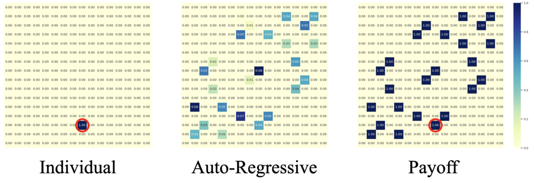
An example of our method deployed on a Clearpath Jackal ground robot (left) exploring a suburban environment to find a visual target (inset). (Right) Egocentric observations of the robot.

Imagine you’re in an unfamiliar neighborhood with no house numbers and I give you a photo that I took a few days ago of my house, which is not too far away. If you tried to find my house, you might follow the streets and go around the block looking for it. You might take a few wrong turns at first, but eventually you would locate my house. In the process, you would end up with a mental map of my neighborhood. The next time you’re visiting, you will likely be able to navigate to my house right away, without taking any wrong turns.

Such exploration and navigation behavior is easy for humans. What would it take for a robotic learning algorithm to enable this kind of intuitive navigation capability? To build a robot capable of exploring and navigating like this, we need to learn from diverse prior datasets in the real world. While it’s possible to collect a large amount of data from demonstrations, or even with randomized exploration, learning meaningful exploration and navigation behavior from this data can be challenging – the robot needs to generalize to unseen neighborhoods, recognize visual and dynamical similarities across scenes, and learn a representation of visual observations that is robust to distractors like weather conditions and obstacles. Since such factors can be hard to model and transfer from simulated environments, we tackle these problems by teaching the robot to explore using only real-world data.

Formally, we studied the problem of goal-directed exploration for visual navigation in novel environments. A robot is tasked with navigating to a goal location , specified by an image taken at . Our method uses an offline dataset of trajectories, over 40 hours of interactions in the real-world, to learn navigational affordances and builds a compressed representation of perceptual inputs. We deploy our method on a mobile robotic system in industrial and recreational outdoor areas around the city of Berkeley. RECON can discover a new goal in a previously unexplored environment in under 10 minutes, and in the process build a “mental map” of that environment that allows it to then reach goals again in just 20 seconds. Additionally, we make this real-world offline dataset publicly available for use in future research.

Rapid Exploration Controllers for Outcome-driven Navigation

RECON, or Rapid Exploration Controllers for Outcome-driven Navigation, explores new environments by “imagining” potential goal images and attempting to reach them. This exploration allows RECON to incrementally gather information about the new environment.

Our method consists of two components that enable it to explore new environments. The first component is a learned representation of goals. This representation ignores task-irrelevant distractors, allowing the agent to quickly adapt to novel settings. The second component is a topological graph. Our method learns both components using datasets or real-world robot interactions gathered in prior work. Leveraging such large datasets allows our method to generalize to new environments and scale beyond the original dataset.

Learning to Represent Goals

A useful strategy to learn complex goal-reaching behavior in an unsupervised manner is for an agent to set its own goals, based on its capabilities, and attempt to reach them. In fact, humans are very proficient at setting abstract goals for themselves in an effort to learn diverse skills. Recent progress in reinforcement learning and robotics has also shown that teaching agents to set its own goals by “imagining” them can result in learning of impressive unsupervised goal-reaching skills. To be able to “imagine”, or sample, such goals, we need to build a prior distribution over the goals seen during training.

For our case, where goals are represented by high-dimensional images, how should we sample goals for exploration? Instead of explicitly sampling goal images, we instead have the agent learn a compact representation of latent goals, allowing us to perform exploration by sampling new latent goal representations, rather than by sampling images. This representation of goals is learned from context-goal pairs previously seen by the robot. We use a variational information bottleneck to learn these representations because it provides two important properties. First, it learns representations that throw away irrelevant information, such as lighting and pixel noise. Second, the variational information bottleneck packs the representations together so that they look like a chosen prior distribution. This is useful because we can then sample imaginary representations by sampling from this prior distribution.

The architecture for learning a prior distribution for these representations is shown below. As the encoder and decoder are conditioned on the context, the representation only encodes information about relative location of the goal from the context – this allows the model to represent feasible goals. If, instead, we had a typical VAE (in which the input images are autoencoded), the samples from the prior over these representations would not necessarily represent goals that are reachable from the current state. This distinction is crucial when exploring new environments, where most states from the training environments are not valid goals.

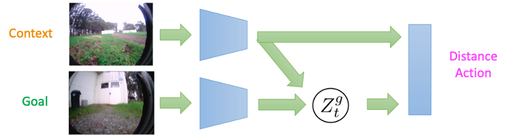
The architecture for learning a prior over goals in RECON. The context-conditioned embedding learns to represent feasible goals.

To understand the importance of learning this representation, we run a simple experiment where the robot is asked to explore in an undirected manner starting from the yellow circle in the figure below. We find that sampling representations from the learned prior greatly accelerates the diversity of exploration trajectories and allows a wider area to be explored. In the absence of a prior over previously seen goals, using random actions to explore the environment can be quite inefficient. Sampling from the prior distribution and attempting to reach these “imagined” goals allows RECON to explore the environment efficiently.

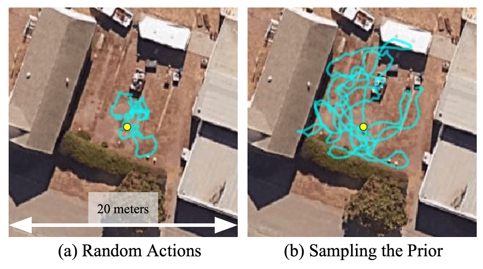
Sampling from a learned prior allows the robot to explore 5 times faster than using random actions.

Goal-Directed Exploration with a Topological Memory

We combine this goal sampling scheme with a topological memory to incrementally build a “mental map” of the new environment. This map provides an estimate of the exploration frontier as well as guidance for subsequent exploration. In a new environment, RECON encourages the robot to explore at the frontier of the map – while the robot is not at the frontier, RECON directs it to navigate to a previously seen subgoal at the frontier of the map.

At the frontier, RECON uses the learned goal representation to learn a prior over goals it can reliably navigate to and are thus, feasible to reach. RECON uses this goal representation to sample, or “imagine”, a feasible goal that helps it explore the environment. This effectively means that, when placed in a new environment, if RECON does not know where the target is, it “imagines” a suitable subgoal that it can drive towards to explore and collects information, until it believes it can reach the target goal image. This allows RECON to “search” for the goal in an unknown environment, all the while building up its mental map. Note that the objective of the topological graph is to build a compact map of the environment and encourage the robot to reach the frontier; it does not inform goal sampling once the robot is at the frontier.

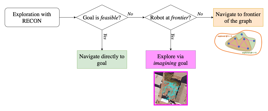
Illustration of the exploration algorithm of RECON.

Learning from Diverse Real-world Data

We train these models in RECON entirely using offline data collected in a diverse range of outdoor environments. Interestingly, we were able to train this model using data collected for two independent projects in the fall of 2019 and spring of 2020, and were successful in deploying the model to explore novel environments and navigate to goals during late 2020 and the spring of 2021. This offline dataset of trajectories consists of over 40 hours of data, including off-road navigation, driving through parks in Berkeley and Oakland, parking lots, sidewalks and more, and is an excellent example of noisy real-world data with visual distractors like lighting, seasons (rain, twilight etc.), dynamic obstacles etc. The dataset consists of a mixture of teleoperated trajectories (2-3 hours) and open-loop safety controllers programmed to collect random data in a self-supervised manner. This dataset presents an exciting benchmark for robotic learning in real-world environments due to the challenges posed by offline learning of control, representation learning from high-dimensional visual observations, generalization to out-of-distribution environments and test-time adaptation.

We are releasing this dataset publicly to support future research in machine learning from real-world interaction datasets, check out the dataset page for more information.

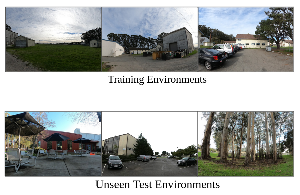
We train from diverse offline data (top) and test in new environments (bottom).

RECON in Action

Putting these components together, let’s see how RECON performs when deployed in a park near Berkeley. Note that the robot has never seen images from this park before. We placed the robot in a corner of the park and provided a target image of a white cabin door. In the animation below, we see RECON exploring and successfully finding the desired goal. “Run 1” corresponds to the exploration process in a novel environment, guided by a user-specified target image on the left. After it finds the goal, RECON uses the mental map to distill its experience in the environment to find the shortest path for subsequent traversals. In “Run 2”, RECON follows this path to navigate directly to the goal without looking around.

In “Run 1”, RECON explores a new environment and builds a topological mental map. In “Run 2”, it uses this mental map to quickly navigate to a user-specified goal in the environment.

An illustration of this two-step process from an overhead view is show below, showing the paths taken by the robot in subsequent traversals of the environment:

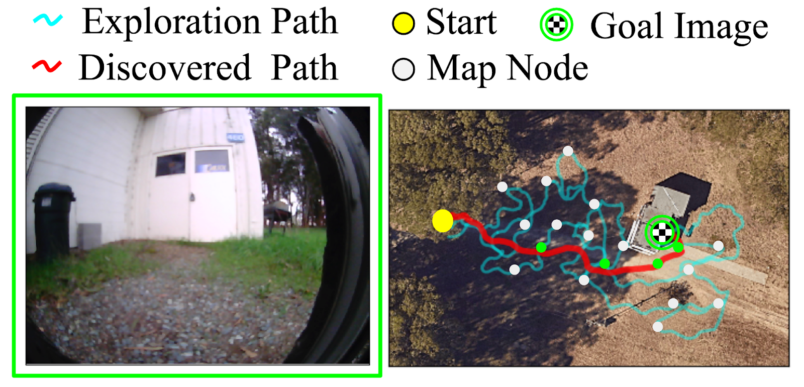
(Left) The goal specified by the user. (Right) The path taken by the robot when exploring for the first time (shown in cyan) to build a mental map with nodes (shown in white), and the path it takes when revisiting the same goal using the mental map (shown in red).

Deploying in Novel Environments

To evaluate the performance of RECON in novel environments, study its behavior under a range of perturbations and understand the contributions of its components, we run extensive real-world experiments in the hills of Berkeley and Richmond, which have a diverse terrain and a wide variety of testing environments.

We compare RECON to five baselines – RND, InfoBot, Active Neural SLAM, ViNG and Episodic Curiosity – each trained on the same offline trajectory dataset as our method, and fine-tuned in the target environment with online interaction. Note that this data is collected from past environments and contains no data from the target environment. The figure below shows the trajectories taken by the different methods for one such environment.

We find that only RECON (and a variant) is able to successfully discover the goal in over 30 minutes of exploration, while all other baselines result in collision (see figure for an overhead visualization). We visualize successful trajectories discovered by RECON in four other environments below.

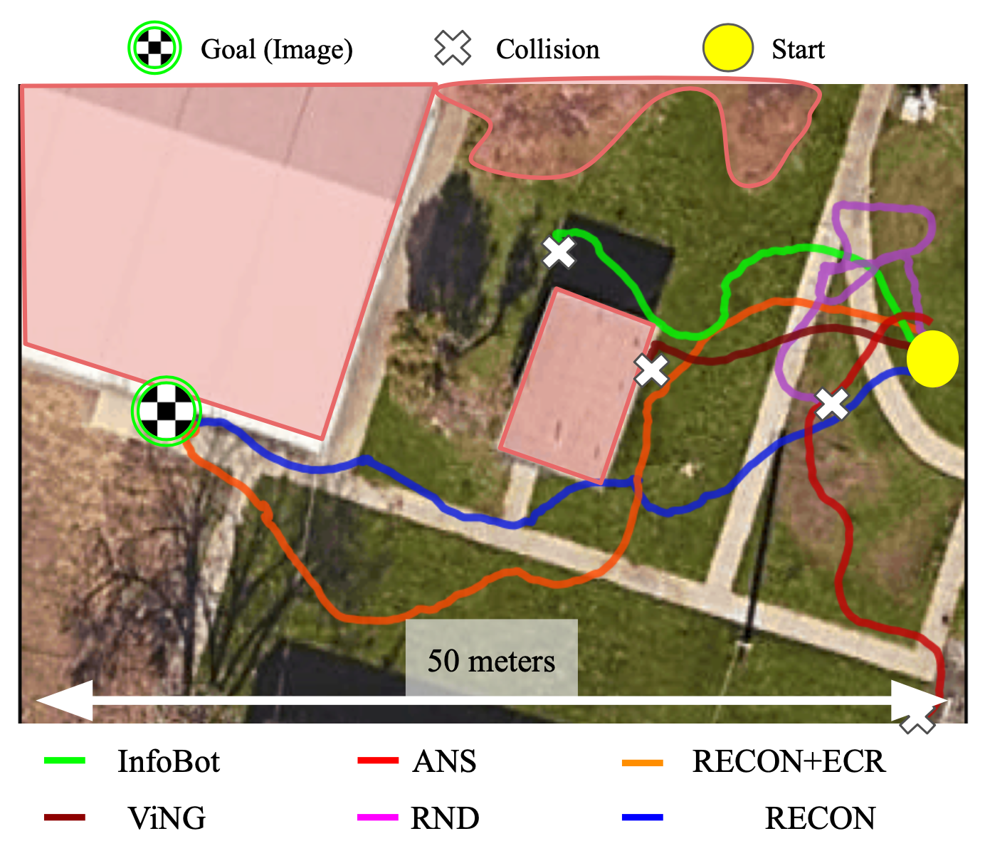
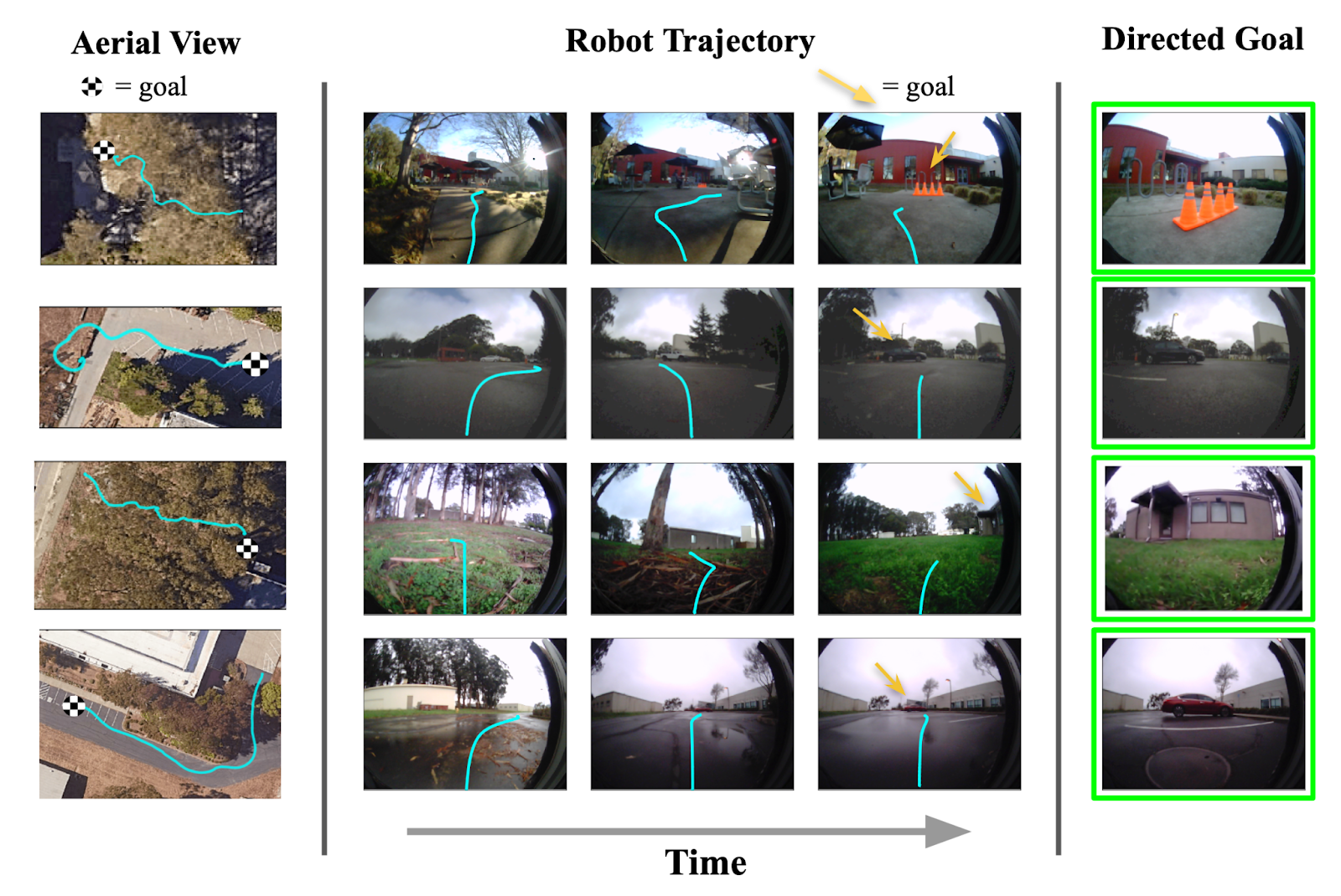
(Top) When comparing to other baselines, only RECON is able to successfully find the goal. (Bottom) Trajectories to goals in four other environments discovered by RECON.

Quantitatively, we observe that our method finds goals over 50% faster than the best prior method; after discovering the goal and building a topological map of the environment, it can navigate to goals in that environment over 25% faster than the best alternative method.

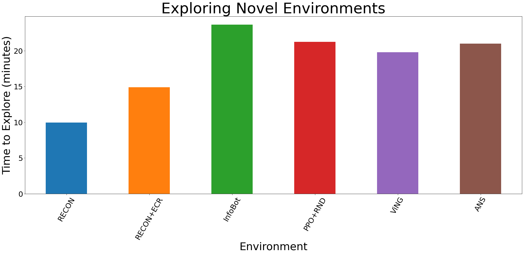
Quantitative results in novel environments. RECON outperforms all baselines by over 50%.

Exploring Non-Stationary Environments

One of the important challenges in designing real-world robotic navigation systems is handling differences between training scenarios and testing scenarios. Typically, systems are developed in well-controlled environments, but are deployed in less structured environments. Further, the environments where robots are deployed often change over time, so tuning a system to perform well on a cloudy day might degrade performance on a sunny day. RECON uses explicit representation learning in attempts to handle this sort of non-stationary dynamics.

Our final experiment tested how changes in the environment affected the performance of RECON. We first had RECON explore a new “junkyard” to learn to reach a blue dumpster. Then, without any more supervision or exploration, we evaluated the learned policy when presented with previously unseen obstacles (trash cans, traffic cones, a car) and weather conditions (sunny, overcast, twilight). As shown below, RECON is able to successfully navigate to the goal in these scenarios, showing that the learned representations are invariant to visual distractors that do not affect the robot’s decisions to reach the goal.

First-person videos of RECON successfully navigating to a “blue dumpster” in the presence of novel obstacles (above) and varying weather conditions (below).

What’s Next?

The problem setup studied in this paper – using past experience to accelerate learning in a new environment – is reflective of several real-world robotics scenarios. RECON provides a robust way to solve this problem by using a combination of goal sampling and topological memory.

A mobile robot capable of reliably exploring and visually observing real-world environments can be a great tool for a wide variety of useful applications such as search and rescue, inspecting large offices or warehouses, finding leaks in oil pipelines or making rounds at a hospital, delivering mail in suburban communities. We demonstrated simplified versions of such applications in an earlier project, where the robot has prior experience in the deployment environment; RECON enables these results to scale beyond the training set of environments and results in a truly open-world learning system that can adapt to novel environments on deployment.

We are also releasing the aforementioned offline trajectory dataset, with hours of real-world interaction of a mobile ground robot in a variety of outdoor environments. We hope that this dataset can support future research in machine learning using real-world data for visual navigation applications. The dataset is also a rich source of sequential data from a multitude of sensors and can be used to test sequence prediction models including, but not limited to, video prediction, LiDAR, GPS etc. More information about the dataset can be found in the full-text article.

This blog post is based on our paper Rapid Exploration for Open-World Navigation with Latent Goal Models, which will be presented as an Oral Talk at the 5th Annual Conference on Robot Learning in London, UK on November 8-11, 2021. You can find more information about our results and the dataset release on the project page.

Big thanks to Sergey Levine and Benjamin Eysenbach for helpful comments on an earlier draft of this article.

Diagram of MURAL, our method for learning uncertainty-aware rewards for RL. After the user provides a few examples of desired outcomes, MURAL automatically infers a reward function that takes into account these examples and the agent’s uncertainty for each state.

Although reinforcement learning has shown success in domains such as robotics, chip placement and playing video games, it is usually intractable in its most general form. In particular, deciding when and how to visit new states in the hopes of learning more about the environment can be challenging, especially when the reward signal is uninformative. These questions of reward specification and exploration are closely connected — the more directed and “well shaped” a reward function is, the easier the problem of exploration becomes. The answer to the question of how to explore most effectively is likely to be closely informed by the particular choice of how we specify rewards.

For unstructured problem settings such as robotic manipulation and navigation — areas where RL holds substantial promise for enabling better real-world intelligent agents — reward specification is often the key factor preventing us from tackling more difficult tasks. The challenge of effective reward specification is two-fold: we require reward functions that can be specified in the real world without significantly instrumenting the environment, but also effectively guide the agent to solve difficult exploration problems. In our recent work, we address this challenge by designing a reward specification technique that naturally incentivizes exploration and enables agents to explore environments in a directed way.

Outcome Driven RL and Classifier Based Rewards

While RL in its most general form can be quite difficult to tackle, we can consider a more controlled set of subproblems which are more tractable while still encompassing a significant set of interesting problems. In particular, we consider a subclass of problems which has been referred to as outcome driven RL. In outcome driven RL problems, the agent is not simply tasked with exploring the environment until it chances upon reward, but instead is provided with examples of successful outcomes in the environment. These successful outcomes can then be used to infer a suitable reward function that can be optimized to solve the desired problems in new scenarios.

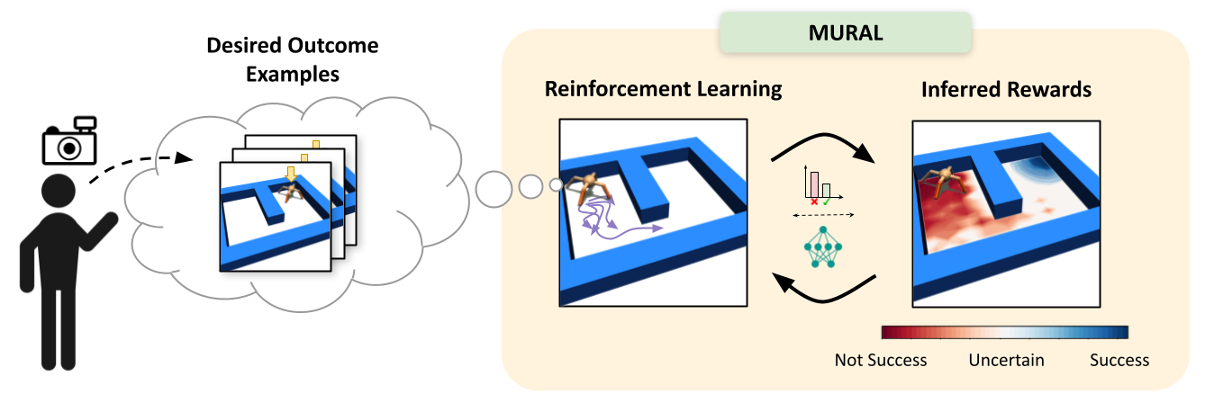
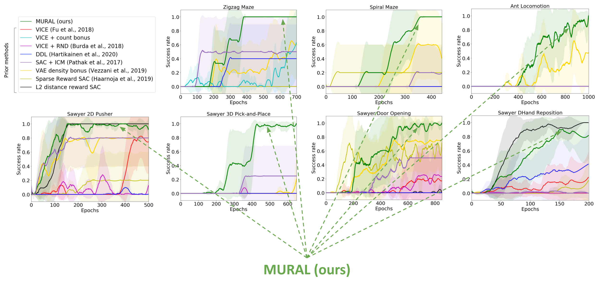
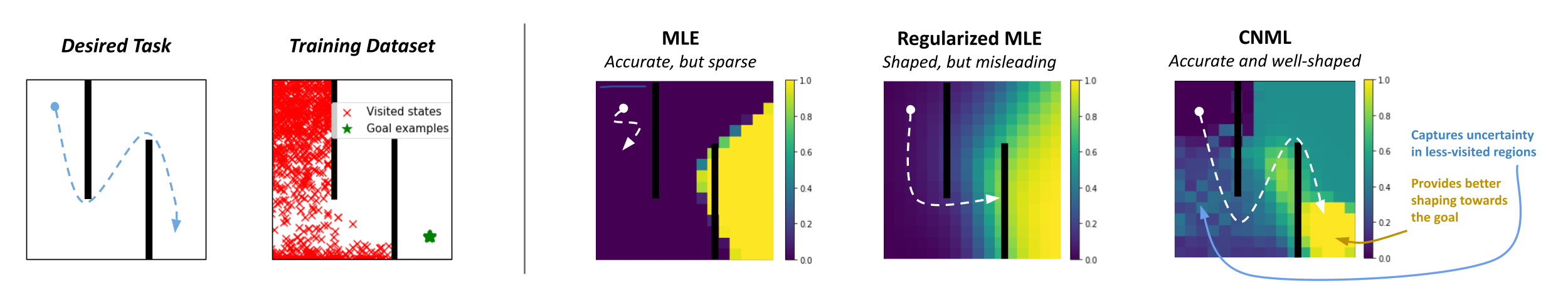
More concretely, in outcome driven RL problems, a human supervisor first provides a set of successful outcome examples , representing states in which the desired task has been accomplished. Given these outcome examples, a suitable reward function can be inferred that encourages an agent to achieve the desired outcome examples. In many ways, this problem is analogous to that of inverse reinforcement learning, but only requires examples of successful states rather than full expert demonstrations.

When thinking about how to actually infer the desired reward function from successful outcome examples , the simplest technique that comes to mind is to simply treat the reward inference problem as a classification problem – “Is the current state a successful outcome or not?” Prior work has implemented this intuition, inferring rewards by training a simple binary classifier to distinguish whether a particular state is a successful outcome or not, using the set of provided goal states as positives, and all on-policy samples as negatives. The algorithm then assigns rewards to a particular state using the success probabilities from the classifier. This has been shown to have a close connection to the framework of inverse reinforcement learning.

Classifier-based methods provide a much more intuitive way to specify desired outcomes, removing the need for hand-designed reward functions or demonstrations:

These classifier-based methods have achieved promising results on robotics tasks such as fabric placement, mug pushing, bead and screw manipulation, and more. However, these successes tend to be limited to simple shorter-horizon tasks, where relatively little exploration is required to find the goal.

What’s Missing?

Standard success classifiers in RL suffer from the key issue of overconfidence, which prevents them from providing useful shaping for hard exploration tasks. To understand why, let’s consider a toy 2D maze environment where the agent must navigate in a zigzag path from the top left to the bottom right corner. During training, classifier-based methods would label all on-policy states as negatives and user-provided outcome examples as positives. A typical neural network classifier would easily assign success probabilities of 0 to all visited states, resulting in uninformative rewards in the intermediate stages when the goal has not been reached.

Since such rewards would not be useful for guiding the agent in any particular direction, prior works tend to regularize their classifiers using methods like weight decay or mixup, which allow for more smoothly increasing rewards as we approach the successful outcome states. However, while this works on many shorter-horizon tasks, such methods can actually produce very misleading rewards. For example, on the 2D maze, a regularized classifier would assign relatively high rewards to states on the opposite side of the wall from the true goal, since they are close to the goal in x-y space. This causes the agent to get stuck in a local optima, never bothering to explore beyond the final wall!

In fact, this is exactly what happens in practice:

Uncertainty-Aware Rewards through CNML

As discussed above, the key issue with unregularized success classifiers for RL is overconfidence — by immediately assigning rewards of 0 to all visited states, we close off many paths that might eventually lead to the goal. Ideally, we would like our classifier to have an appropriate notion of uncertainty when outputting success probabilities, so that we can avoid excessively low rewards without suffering from the misleading local optima that result from regularization.

Conditional Normalized Maximum Likelihood (CNML)

One method particularly well-suited for this task is Conditional Normalized Maximum Likelihood (CNML). The concept of normalized maximum likelihood (NML) has typically been used in the Bayesian inference literature for model selection, to implement the minimum description length principle. In more recent work, NML has been adapted to the conditional setting to produce models that are much better calibrated and maintain a notion of uncertainty, while achieving optimal worst case classification regret. Given the challenges of overconfidence described above, this is an ideal choice for the problem of reward inference.

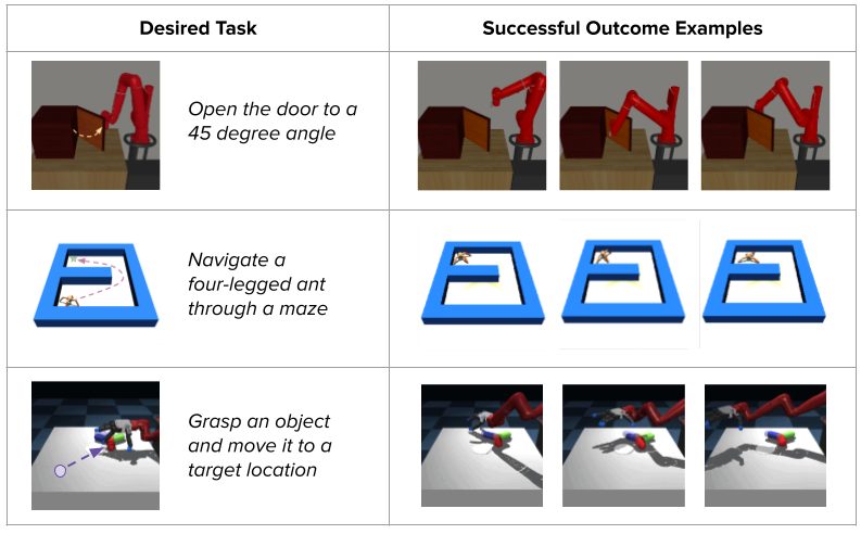
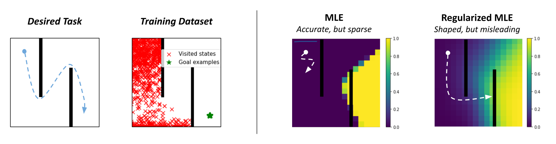
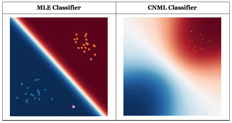
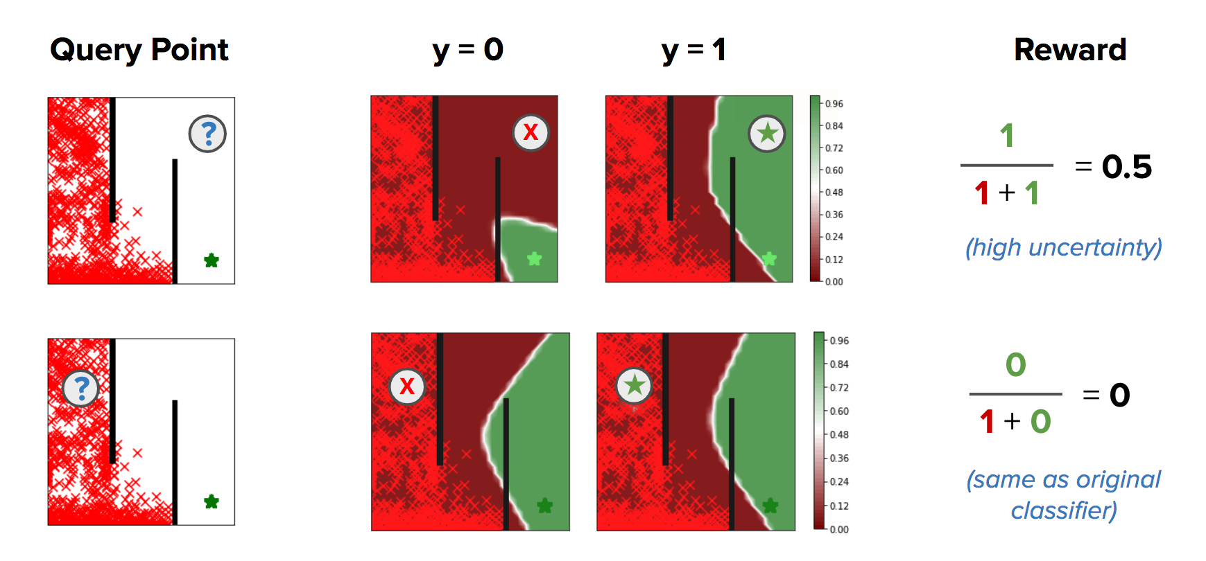
Rather than simply training models via maximum likelihood, CNML performs a more complex inference procedure to produce likelihoods for any point that is being queried for its label. Intuitively, CNML constructs a set of different maximum likelihood problems by labeling a particular query point with every possible label value that it might take, then outputs a final prediction based on how easily it was able to adapt to each of those proposed labels given the entire dataset observed thus far. Given a particular query point , and a prior dataset , CNML solves k different maximum likelihood problems and normalizes them to produce the desired label likelihood , where represents the number of possible values that the label may take. Formally, given a model , loss function , training dataset with classes , and a new query point , CNML solves the following maximum likelihood problems:

It then generates predictions for each of the classes using their corresponding models, and normalizes the results for its final output:

Comparison of outputs from a standard classifier and a CNML classifier. CNML outputs more conservative predictions on points that are far from the training distribution, indicating uncertainty about those points’ true outputs. (Credit: Aurick Zhou, BAIR Blog)

Intuitively, if the query point is farther from the original training distribution represented by D, CNML will be able to more easily adapt to any arbitrary label in , making the resulting predictions closer to uniform. In this way, CNML is able to produce better calibrated predictions, and maintain a clear notion of uncertainty based on which data point is being queried.

Leveraging CNML-based classifiers for Reward Inference

Given the above background on CNML as a means to produce better calibrated classifiers, it becomes clear that this provides us a straightforward way to address the overconfidence problem with classifier based rewards in outcome driven RL. By replacing a standard maximum likelihood classifier with one trained using CNML, we are able to capture a notion of uncertainty and obtain directed exploration for outcome driven RL. In fact, in the discrete case, CNML corresponds to imposing a uniform prior on the output space — in an RL setting, this is equivalent to using a count-based exploration bonus as the reward function. This turns out to give us a very appropriate notion of uncertainty in the rewards, and solves many of the exploration challenges present in classifier based RL.

However, we don’t usually operate in the discrete case. In most cases, we use expressive function approximators and the resulting representations of different states in the world share similarities. When a CNML based classifier is learned in this scenario, with expressive function approximation, we see that it can provide more than just task agnostic exploration. In fact, it can provide a directed notion of reward shaping, which guides an agent towards the goal rather than simply encouraging it to expand the visited region naively. As visualized below, CNML encourages exploration by giving optimistic success probabilities in less-visited regions, while also providing better shaping towards the goal.

As we will show in our experimental results, this intuition scales to higher dimensional problems and more complex state and action spaces, enabling CNML based rewards to solve significantly more challenging tasks than is possible with typical classifier based rewards.

However, on closer inspection of the CNML procedure, a major challenge becomes apparent. Each time a query is made to the CNML classifier, different maximum likelihood problems need to be solved to convergence, then normalized to produce the desired likelihood. As the size of the dataset increases, as it naturally does in reinforcement learning, this becomes a prohibitively slow process. In fact, as seen in Table 1, RL with standard CNML based rewards takes around 4 hours to train a single epoch (1000 timesteps). Following this procedure blindly would take over a month to train a single RL agent, necessitating a more time efficient solution. This is where we find meta-learning to be a crucial tool.

Meta-Learning CNML Classifiers

Meta-learning is a tool that has seen a lot of use cases in few-shot learning for image classification, learning quicker optimizers and even learning more efficient RL algorithms. In essence, the idea behind meta-learning is to leverage a set of “meta-training” tasks to learn a model (and often an adaptation procedure) that can very quickly adapt to a new task drawn from the same distribution of problems.

Meta-learning techniques are particularly well suited to our class of computational problems since it involves quickly solving multiple different maximum likelihood problems to evaluate the CNML likelihood. Each the maximum likelihood problems share significant similarities with each other, enabling a meta-learning algorithm to very quickly adapt to produce solutions for each individual problem. In doing so, meta-learning provides us an effective tool for producing estimates of normalized maximum likelihood significantly more quickly than possible before.

The intuition behind how to apply meta-learning to the CNML (meta-NML) can be understood by the graphic above. For a data-set of points, meta-NML would first construct tasks, corresponding to the positive and negative maximum likelihood problems for each datapoint in the dataset. Given these constructed tasks as a (meta) training set, a meta–learning algorithm can be applied to learn a model that can very quickly be adapted to produce solutions to any of these maximum likelihood problems. 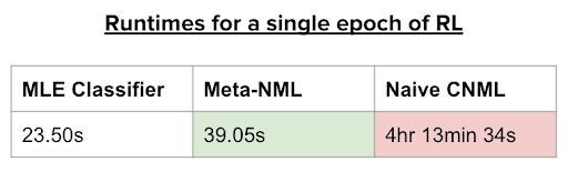Equipped with this scheme to very quickly solve maximum likelihood problems, producing CNML predictions around x faster than possible before. Prior work studied this problem from a Bayesian approach, but we found that it often scales poorly for the problems we considered.

Equipped with a tool for efficiently producing predictions from the CNML distribution, we can now return to the goal of solving outcome-driven RL with uncertainty aware classifiers, resulting in an algorithm we call MURAL.

MURAL: Meta-Learning Uncertainty-Aware Rewards for Automated Reinforcement Learning

To more effectively solve outcome driven RL problems, we incorporate meta-NML into the standard classifier based procedure as follows: After each epoch of RL, we sample a batch of points from the replay buffer and use them to construct meta-tasks. We then run iteration of meta-training on our model.
We assign rewards using NML, where the NML outputs are approximated using only one gradient step for each input point.

The resulting algorithm, which we call MURAL, replaces the classifier portion of standard classifier-based RL algorithms with a meta-NML model instead. Although meta-NML can only evaluate input points one at a time instead of in batches, it is substantially faster than naive CNML, and MURAL is still comparable in runtime to standard classifier-based RL, as shown in Table 1 below.

Table 1. Runtimes for a single epoch of RL on the 2D maze task.

We evaluate MURAL on a variety of navigation and robotic manipulation tasks, which present several challenges including local optima and difficult exploration. MURAL solves all of these tasks successfully, outperforming prior classifier-based methods as well as standard RL with exploration bonuses.

Visualization of behaviors learned by MURAL. MURAL is able to perform a variety of behaviors in navigation and manipulation tasks, inferring rewards from outcome examples.

Quantitative comparison of MURAL to baselines. MURAL is able to outperform baselines which perform task-agnostic exploration, standard maximum likelihood classifiers.

This suggests that using meta-NML based classifiers for outcome driven RL provides us an effective way to provide rewards for RL problems, providing benefits both in terms of exploration and directed reward shaping.

Takeaways

In conclusion, we showed how outcome driven RL can define a class of more tractable RL problems. Standard methods using classifiers can often fall short in these settings as they are unable to provide any benefits of exploration or guidance towards the goal. Leveraging a scheme for training uncertainty aware classifiers via conditional normalized maximum likelihood allows us to more effectively solve this problem, providing benefits in terms of exploration and reward shaping towards successful outcomes. The general principles defined in this work suggest that considering tractable approximations to the general RL problem may allow us to simplify the challenge of reward specification and exploration in RL while still encompassing a rich class of control problems.

This post is based on the paper “MURAL: Meta-Learning Uncertainty-Aware Rewards for Outcome-Driven Reinforcement Learning”, which was presented at ICML 2021. You can see results on our website, and we provide code to reproduce our experiments.

How do humans become so skillful? Well, initially we are not, but from infancy, we discover and practice increasingly complex skills through self-supervised play. But this play is not random – the child development literature suggests that infants use their prior experience to conduct directed exploration of affordances like movability, suckability, graspability, and digestibility through interaction and sensory feedback. This type of affordance directed exploration allows infants to learn both what can be done in a given environment and how to do it. Can we instantiate an analogous strategy in a robotic learning system?

On the left we see videos from a prior dataset collected with a robot accomplishing various tasks such as drawer opening and closing, as well as grasping and relocating objects. On the right we have a lid that the robot has never seen before. The robot has been granted a short period of time to practice with the new object, after which it will be given a goal image and tasked with making the scene match this image. How can the robot rapidly learn to manipulate the environment and grasp this lid without any external supervision?

Read More

By Ben Eysenbach

Nearly all real-world applications of reinforcement learning involve some degree of shift between the training environment and the testing environment. However, prior work has observed that even small shifts in the environment cause most RL algorithms to perform markedly worse. As we aim to scale reinforcement learning algorithms and apply them in the real world, it is increasingly important to learn policies that are robust to changes in the environment.

Robust reinforcement learning maximizes reward on an adversarially-chosen environment.

Broadly, prior approaches to handling distribution shift in RL aim to maximize performance in either the average case or the worst case. The first set of approaches, such as domain randomization, train a policy on a distribution of environments, and optimize the average performance of the policy on these environments. While these methods have been successfully applied to a number of areas (e.g., self-driving cars, robot locomotion and manipulation), their success rests critically on the design of the distribution of environments. Moreover, policies that do well on average are not guaranteed to get high reward on every environment. The policy that gets the highest reward on average might get very low reward on a small fraction of environments. The second set of approaches, typically referred to as robust RL, focus on the worst-case scenarios. The aim is to find a policy that gets high reward on every environment within some set. Robust RL can equivalently be viewed as a two-player game between the policy and an environment adversary. The policy tries to get high reward, while the environment adversary tries to tweak the dynamics and reward function of the environment so that the policy gets lower reward. One important property of the robust approach is that, unlike domain randomization, it is invariant to the ratio of easy and hard tasks. Whereas robust RL always evaluates a policy on the most challenging tasks, domain randomization will predict that the policy is better if it is evaluated on a distribution of environments with more easy tasks.

Prior work has suggested a number of algorithms for solving robust RL problems. Generally, these algorithms all follow the same recipe: take an existing RL algorithm and add some additional machinery on top to make it robust. For example, robust value iteration uses Q-learning as the base RL algorithm, and modifies the Bellman update by solving a convex optimization problem in the inner loop of each Bellman backup. Similarly, Pinto ‘17 uses TRPO as the base RL algorithm and periodically updates the environment based on the behavior of the current policy. These prior approaches are often difficult to implement and, even once implemented correctly, they requiring tuning of many additional hyperparameters. Might there be a simpler approach, an approach that does not require additional hyperparameters and additional lines of code to debug?

To answer this question, we are going to focus on a type of RL algorithm known as maximum entropy RL, or MaxEnt RL for short (Todorov ‘06, Rawlik ‘08, Ziebart ‘10). MaxEnt RL is a slight variant of standard RL that aims to learn a policy that gets high reward while acting as randomly as possible; formally, MaxEnt maximizes the entropy of the policy. Some prior work has observed empirically that MaxEnt RL algorithms appear to be robust to some disturbances the environment. To the best of our knowledge, no prior work has actually proven that MaxEnt RL is robust to environmental disturbances.

In a recent paper, we prove that every MaxEnt RL problem corresponds to maximizing a lower bound on a robust RL problem. Thus, when you run MaxEnt RL, you are implicitly solving a robust RL problem. Our analysis provides a theoretically-justified explanation for the empirical robustness of MaxEnt RL, and proves that MaxEnt RL is itself a robust RL algorithm. In the rest of this post, we’ll provide some intuition into why MaxEnt RL should be robust and what sort of perturbations MaxEnt RL is robust to. We’ll also show some experiments demonstrating the robustness of MaxEnt RL.

Intuition

So, why would we expect MaxEnt RL to be robust to disturbances in the environment? Recall that MaxEnt RL trains policies to not only maximize reward, but to do so while acting as randomly as possible. In essence, the policy itself is injecting as much noise as possible into the environment, so it gets to “practice” recovering from disturbances. Thus, if the change in dynamics appears like just a disturbance in the original environment, our policy has already been trained on such data. Another way of viewing MaxEnt RL is as learning many different ways of solving the task (Kappen ‘05). For example, let’s look at the task shown in videos below: we want the robot to push the white object to the green region. The top two videos show that standard RL always takes the shortest path to the goal, whereas MaxEnt RL takes many different paths to the goal. Now, let’s imagine that we add a new obstacle (red blocks) that wasn’t included during training. As shown in the videos in the bottom row, the policy learned by standard RL almost always collides with the obstacle, rarely reaching the goal. In contrast, the MaxEnt RL policy often chooses routes around the obstacle, continuing to reach the goal for a large fraction of trials.

	Standard RL	MaxEnt RL
Trained and evaluated without the obstacle:
Trained without the obstacle, but evaluated with the obstacle:

Theory

We now formally describe the technical results from the paper. The aim here is not to provide a full proof (see the paper Appendix for that), but instead to build some intuition for what the technical results say. Our main result is that, when you apply MaxEnt RL with some reward function and some dynamics, you are actually maximizing a lower bound on the robust RL objective. To explain this result, we must first define the MaxEnt RL objective: $J_{MaxEnt}(\pi; p, r)$ is the entropy-regularized cumulative return of policy $\pi$ when evaluated using dynamics $p(s’ \mid s, a)$ and reward function $r(s, a)$. While we will train the policy using one dynamics $p$, we will evaluate the policy on a different dynamics, $\tilde{p}(s’ \mid s, a)$, chosen by the adversary. We can now formally state our main result as follows:

$$\min_{\tilde{p} \in \tilde{\mathcal{P}}(\pi)} J_\text{MaxEnt}(\pi; \tilde{p}, r) \ge \exp(J_\text{MaxEnt}(\pi; p, \bar{r}) + \log T.$$

The left-hand-side is the robust RL objective. It says that the adversary gets to choose whichever dynamics function $\tilde{p}(s’ \mid s, a)$ makes our policy perform as poorly as possible, subject to some constraints (as specified by the set $\tilde{\mathcal{P}}$). On the right-hand-side we have the MaxEnt RL objective (note that $\log T$ is a constant, and the function $\exp(\cdots)$ is always increasing). Thus, this objective says that a policy that has a high entropy-regularized reward (right hand-side) is guaranteed to also get high reward when evaluated on an adversarially-chosen dynamics.

The most important part of this equation is the set $\tilde{\mathcal{P}}$ of dynamics that the adversary can choose from. Our analysis describes precisely how this set is constructed and shows that, if we want a policy to be robust to a larger set of disturbances, all we have to do is increase the weight on the entropy term and decrease the weight on the reward term. Intuitively, the adversary must choose dynamics that are “close” to the dynamics on which the policy was trained. For example, in the special case where the dynamics are linear-Gaussian, this set corresponds to all perturbations where the original expected next state and the perturbed expected next state have a Euclidean distance less than $\epsilon$.

More Experiments

Our analysis predicts that MaxEnt RL should be robust to many types of disturbances. The first set of videos in this post showed that MaxEnt RL is robust to static obstacles. MaxEnt RL is also robust to dynamic perturbations introduced in the middle of an episode. To demonstrate this, we took the same robotic pushing task and knocked the puck out of place in the middle of the episode. The videos below show that the policy learned by MaxEnt RL is more robust at handling these perturbations, as predicted by our analysis.

Standard RL	MaxEnt RL

The policy learned by MaxEntRL is robust to dynamic perturbations of the puck (red frames).

Our theoretical results suggest that, even if we optimize the environment perturbations so the agent does as poorly as possible, MaxEnt RL policies will still be robust. To demonstrate this capability, we trained both standard RL and MaxEnt RL on a peg insertion task shown below. During evaluation, we changed the position of the hole to try to make each policy fail. If we only moved the hole position a little bit ($\le$ 1 cm), both policies always solved the task. However, if we moved the hole position up to 2cm, the policy learned by standard RL almost never succeeded in inserting the peg, while the MaxEnt RL policy succeeded in 95% of trials. This experiment validates our theoretical findings that MaxEnt really is robust to (bounded) adversarial disturbances in the environment.

Standard RL	MaxEnt RL	Evaluation on adversarial perturbations

MaxEnt RL is robust to adversarial perturbations of the hole (where the robot
inserts the peg).

Conclusion

In summary, our paper shows that a commonly-used type of RL algorithm, MaxEnt RL, is already solving a robust RL problem. We do not claim that MaxEnt RL will outperform purpose-designed robust RL algorithms. However, the striking simplicity of MaxEnt RL compared with other robust RL algorithms suggests that it may be an appealing alternative to practitioners hoping to equip their RL policies with an ounce of robustness.

Acknowledgements
Thanks to Gokul Swamy, Diba Ghosh, Colin Li, and Sergey Levine for feedback on drafts of this post, and to Chloe Hsu and Daniel Seita for help with the blog.

This post is based on the following paper:

• Maximum Entropy RL (Provably) Solves Some Robust RL Problems.
  Benjamin Eysenbach and Sergey Levine.

Our method learns a task in a fixed, simulated environment and quickly adapts
to new environments (e.g. the real world) solely from online interaction during
deployment.

The ability for humans to generalize their knowledge and experiences to new situations is remarkable, yet poorly understood. For example, imagine a human driver that has only ever driven around their city in clear weather. Even though they never encountered true diversity in driving conditions, they have acquired the fundamental skill of driving, and can adapt reasonably fast to driving in neighboring cities, in rainy or windy weather, or even driving a different car, without much practice nor additional driver’s lessons. While humans excel at adaptation, building intelligent systems with common-sense knowledge and the ability to quickly adapt to new situations is a long-standing problem in artificial intelligence.

A robot trained to perform a given task in a lab environment may not generalize
to other environments, e.g. an environment with moving disco lights, even
though the task itself remains the same.

In recent years, learning both perception and behavioral policies in an end-to-end framework by deep Reinforcement Learning (RL) has been widely successful, and has achieved impressive results such as superhuman performance on Atari games played directly from screen pixels. Although impressive, it has become commonly understood that such policies fail to generalize to even subtle changes in the environment – changes that humans are easily able to adapt to. For this reason, RL has shown limited success beyond the game or environment in which it was originally trained, which presents a significant challenge in deployment of policies trained by RL in our diverse and unstructured real world.

Generalization by Randomization

In applications of RL, practitioners have sought to improve the generalization ability of policies by introducing randomization into the training environment (e.g. a simulation), also known as domain randomization. By randomizing elements of the training environment that are also expected to vary at test-time, it is possible to learn policies that are invariant to certain factors of variation. For autonomous driving, we may for example want our policy to be robust to changes in lighting, weather, and road conditions, as well as car models, nearby buildings, different city layouts, and so forth. While the randomization quickly evolves into an elaborate engineering challenge as more and more factors of variation are considered, the learning problem itself also becomes harder, greatly decreasing the sample efficiency of learning algorithms. It is therefore natural to ask: rather than learning a policy robust to all conceivable environmental changes, can we instead adapt a pre-trained policy to the new environment through interaction?

Left: training in a fixed environment. Right: training with
domain randomization.

Policy Adaptation

A naïve way to adapt a policy to new environments is by fine-tuning parameters using a reward signal. In real-world deployments, however, obtaining a reward signal often requires human feedback or careful engineering, neither of which are scalable solutions.

In recent work from our lab, we show that it is possible to adapt a pre-trained policy to unseen environments, without any reward signal or human supervision. A key insight is that, in the context of many deployments of RL, the fundamental goal of the task remains the same, even though there may be a mismatch in both visuals and underlying dynamics compared to the training environment, e.g. a simulation. When training a policy in simulation and deploying it in the real world (sim2real), there are often differences in dynamics due to imperfections in the simulation, and visual inputs captured by a camera are likely to differ from renderings of the simulation. Hence, the source of these errors often lie in an imperfect world understanding rather than misspecification of the task itself, and an agent’s interactions with a new environment can therefore provide us with valuable information about the disparity between its world understanding and reality.

Illustration of our framework for adaptation. Left: training before
deployment. The RL objective is optimized together with a self-supervised
objective. Right: adaptation during deployment. We optimize only the
self-supervised objective, using observations collected through interaction
with the environment.

To take advantage of this information we turn to the literature of self-supervised learning. We propose PAD, a general framework for adaptation of policies during deployment, by using self-supervision as a proxy for the absent reward signal. A given policy network $\pi$ parameterized by a collection of parameters $\theta$ is split sequentially into an encoder $\pi_{e}$ and a policy head $\pi_{a}$ such that $a_{t} = \pi(s_{t}; \theta) = \pi_{a} (\pi_{e}(s_{t}; \theta_{e}) ;\theta_{a})$ for a state $s_{t}$ and action $a_{t}$ at time $t$. We then let $\pi_{s}$ be a self-supervised task head and similarly let $\pi_{s}$ share the encoder $\pi_{e}$ with the policy head. During training, we optimize a self-supervised objective jointly together with the RL task, where the two tasks share part of a neural network. During deployment, we can no longer assume access to a reward signal and are unable to optimize the RL objective. However, we can still continue to optimize the self-supervised objective using observations collected through interaction with the new environment. At every step in the new environment, we update the policy through self-supervision, using only the most recently collected observation:

$$s_t \sim p(s_t | a_{t-1}, s_{t-1}) \\
\theta_{e}(t) = \theta_{e}(t-1) – \nabla_{\theta_{e}}L(s_{t}; \theta_{s}(t-1), \theta_{e}(t-1))$$

where L is a self-supervised objective. Assuming that gradients of the self-supervised objective are sufficiently correlated with those of the RL objective, any adaptation in the self-supervised task may also influence and correct errors in the perception and decision-making of the policy.

In practice, we use an inverse dynamics model $a_{t} = \pi_{s}( \pi_e(s_{t}), \pi_e(s_{t+1}))$, predicting the action taken in between two consecutive observations. Because an inverse dynamics model connects observations directly to actions, the policy can be adjusted for disparities both in visuals and dynamics (e.g. lighting conditions or friction) between training and test environments, solely through interaction with the new environment.

Adapting policies to the real world

We demonstrate the effectiveness of self-supervised policy adaptation (PAD) by training policies for robotic manipulation tasks in simulation and adapting them to the real world during deployment on a physical robot, taking observations directly from an uncalibrated camera. We evaluate generalization to a real robot environment that resembles the simulation, as well as two more challenging settings: a table cloth with increased friction, and continuously moving disco lights. In the demonstration below, we consider a Soft Actor-Critic (SAC) agent trained with an Inverse Dynamics Model (IDM), with and without the PAD adaptation mechanism.

Transferring a policy from simulation to the real world. SAC+IDM is a
Soft Actor-Critic (SAC) policy trained with an Inverse Dynamics Model (IDM),
and SAC+IDM (PAD) is the same policy but with the addition of policy
adaptation during deployment on the robot.

PAD adapts to changes in both visuals and dynamics, and nearly recovers the original success rate of the simulated environment. Policy adaptation is especially effective when the test environment differs from the training environment in multiple ways, e.g. where both visuals and physical properties such as object dimensionality and friction differ. Because it is often difficult to formally specify the elements that vary between a simulation and the real world, policy adaptation may be a promising alternative to domain randomization techniques in such settings.

Benchmarking generalization

Simulations provide a good platform for more comprehensive evaluation of RL algorithms. Together with PAD, we release DMControl Generalization Benchmark, a new benchmark for generalization in RL based on the DeepMind Control Suite, a popular benchmark for continuous control from images. In the DMControl Generalization Benchmark, agents are trained in a fixed environment and deployed in new environments with e.g. randomized colors or continuously changing video backgrounds. We consider an SAC agent trained with an IDM, with and without adaptation, and compare to CURL, a contrastive method discussed in a previous post. We compare the generalization ability of methods in the visualization below, and generally find that PAD can adapt even in non-stationary environments, a challenging problem setting where non-adaptive methods tend to fail. While CURL is found to generalize no better than the non-adaptive SAC trained with an IDM, agents can still benefit from the training signal that CURL provides during the training phase. Algorithms that learn both during training and deployment, and from multiple training signals, may therefore be preferred.

Generalization to an environment with video background. CURL is a
contrastive method, SAC+IDM is a Soft Actor-Critic (SAC) policy trained
with an Inverse Dynamics Model (IDM), and SAC+IDM (PAD) is the same
policy but with the addition of policy adaptation during deployment.

Summary

Previous work addresses the problem of generalization in RL by randomization, which requires anticipation of environmental changes and is known to not scale well. We formulate an alternative problem setting in vision-based RL: can we instead adapt a pre-trained policy to unseen environments, without any rewards or human feedback? We find that adapting policies through a self-supervised objective – solely from interactions in the new environment – is a promising alternative to domain randomization when the target environment is truly unknown. In the future, we ultimately envision agents that continuously learn and adapt to their surroundings, and are capable of learning both from explicit human feedback and through unsupervised interaction with the environment.

This post is based on the following paper:

• Self-Supervised Policy Adaptation during Deployment
  Nicklas Hansen, Rishabh Jangir, Yu Sun, Guillem Alenyá, Pieter Abbeel, Alexei A. Efros, Lerrel Pinto, Xiaolong Wang
  Ninth International Conference on Learning Representations (ICLR), 2021
  arXiv, Project Website, Code

By Oleh Rybkin, Danijar Hafner and Deepak Pathak

To operate successfully in unstructured open-world environments, autonomous intelligent agents need to solve many different tasks and learn new tasks quickly. Reinforcement learning has enabled artificial agents to solve complex tasks both in simulation and real-world. However, it requires collecting large amounts of experience in the environment for each individual task.

Self-supervised reinforcement learning has emerged as an alternative, where the agent only follows an intrinsic objective that is independent of any individual task, analogously to unsupervised representation learning. After acquiring general and reusable knowledge about the environment through self-supervision, the agent can adapt to specific downstream tasks more efficiently.

In this post, we explain our recent publication that develops Plan2Explore. While many recent papers on self-supervised reinforcement learning have focused on model-free agents, our agent learns an internal world model that predicts the future outcomes of potential actions. The world model captures general knowledge, allowing Plan2Explore to quickly solve new tasks through planning in its own imagination. The world model further enables the agent to explore what it expects to be novel, rather than repeating what it found novel in the past. Plan2Explore obtains state-of-the-art zero-shot and few-shot performance on continuous control benchmarks with high-dimensional input images. To make it easy to experiment with our agent, we are open-sourcing the complete source code.

How does Plan2Explore work?

At a high level, Plan2Explore works by training a world model, exploring to maximize the information gain for the world model, and using the world model at test time to solve new tasks (see figure above). Thanks to effective exploration, the learned world model is general and captures information that can be used to solve multiple new tasks with no or few additional environment interactions. We discuss each part of the Plan2Explore algorithm individually below. We assume a basic understanding of reinforcement learning in this post and otherwise recommend these materials as an introduction.

Learning the world model

Plan2Explore learns a world model that predicts future outcomes given past observations $o_{1:t}$ and actions $a_{1:t}$ (see figure below). To handle high-dimensional image observations, we encode them into lower-dimensional features $h$ and use an RSSM model that predicts forward in a compact latent state-space $s$, from which the observations can be decoded. The latent state aggregates information from past observations that is helpful for future prediction, and is learned end-to-end using a variational objective.

A novelty metric for active model-building

To learn an accurate and general world model we need an exploration strategy that collects new and informative data. To achieve this, Plan2Explore uses a novelty metric derived from the model itself. The novelty metric measures the expected information gained about the environment upon observing the new data. As the figure below shows, this is approximated by the disagreement of an ensemble of $K$ latent models. Intuitively, large latent disagreement reflects high model uncertainty, and obtaining the data point would reduce this uncertainty. By maximizing latent disagreement, Plan2Explore selects actions that lead to the largest information gain, therefore improving the model as quickly as possible.

Planning for future novelty

To effectively maximize novelty, we need to know which parts of the environment are still unexplored. Most prior work on self-supervised exploration used model-free methods that reinforce past behavior that resulted in novel experience. This makes these methods slow to explore: since they can only repeat exploration behavior that was successful in the past, they are unlikely to stumble onto something novel. In contrast, Plan2Explore plans for expected novelty by measuring model uncertainty of imagined future outcomes. By seeking trajectories that have the highest uncertainty, Plan2Explore explores exactly the parts of the environments that were previously unknown.

To choose actions $a$ that optimize the exploration objective, Plan2Explore leverages the learned world model as shown in the figure below. The actions are selected to maximize the expected novelty of the entire future sequence $s_{t:T}$, using imaginary rollouts of the world model to estimate the novelty. To solve this optimization problem, we use the Dreamer agent, which learns a policy $\pi_\phi$ using a value function and analytic gradients through the model. The policy is learned completely inside the imagination of the world model. During exploration, this imagination training ensures that our exploration policy is always up-to-date with the current world model and collects data that are still novel.

Curiosity-driven exploration behavior

We evaluate Plan2Explore on 20 continuous control tasks from the DeepMind Control Suite. The agent only has access to image observations and no proprioceptive information. Instead of random exploration, which fails to take the agent far from the initial position, Plan2Explore leads to diverse movement strategies like jumping, running, and flipping. Later, we will see that these are effective practice episodes that enable the agent to quickly learn to solve various continuous control tasks.

Solving tasks with the world model

Once an accurate and general world model is learned, we test Plan2Explore on previously unseen tasks. Given a task specified with a reward function, we use the model to optimize a policy for that task. Similar to our exploration procedure, we optimize a new value function and a new policy head for the downstream task. This optimization uses only predictions imagined by the model, enabling Plan2Explore to solve new downstream tasks in a zero-shot manner without any additional interaction with the world.

The following plot shows the performance of Plan2Explore on tasks from DM Control Suite. Before 1 million environment steps, the agent doesn’t know the task and simply explores. The agent solves the task as soon as it is provided at 1 million steps, and keeps improving fast in a few-shot regime after that.

Plan2Explore (—) is able to solve most of the tasks we benchmarked. Since prior work on self-supervised reinforcement learning used model-free agents that are not able to adapt in a zero-shot manner (ICM, —), or did not use image observations, we compare by adapting this prior work to our model-based plan2explore setup. Our latent disagreement objective outperforms other previously proposed objectives. More interestingly, the final performance of Plan2Explore is comparable to the state-of-the-art oracle agent that requires task rewards throughout training (—). In our paper, we further report performance of Plan2Explore in the zero-shot setting where the agent needs to solve the task before any task-oriented practice.

Future directions

Plan2Explore demonstrates that effective behavior can be learned through self-supervised exploration only. This opens multiple avenues for future research:

• First, to apply self-supervised RL to a variety of settings, future work will investigate different ways of specifying the task and deriving behavior from the world model. For example, the task could be specified with a demonstration, description of the desired goal state, or communicated to the agent in natural language.

• Second, while Plan2Explore is completely self-supervised, in many cases a weak supervision signal is available, such as in hard exploration games, human-in-the-loop learning, or real life. In such a semi-supervised setting, it is interesting to investigate how weak supervision can be used to steer exploration towards the relevant parts of the environment.

• Finally, Plan2Explore has the potential to improve the data efficiency of real-world robotic systems, where exploration is costly and time-consuming, and the final task is often unknown in advance.

By designing a scalable way of planning to explore in unstructured environments with visual observations, Plan2Explore provides an important step toward self-supervised intelligent machines.

We would like to thank Georgios Georgakis for the useful feedback.

This post is based on the following paper:

• Planning to Explore via Self-Supervised World Models
  Ramanan Sekar*, Oleh Rybkin*, Kostas Daniilidis, Pieter Abbeel, Danijar Hafner, Deepak Pathak
  Thirty-seventh International Conference Machine Learning (ICML), 2020.
  arXiv, Project Website

This article was initially published on the BAIR blog, and appears here with the authors’ permission.

By Ashvin Nair and Abhishek Gupta

Robots trained with reinforcement learning (RL) have the potential to be used across a huge variety of challenging real world problems. To apply RL to a new problem, you typically set up the environment, define a reward function, and train the robot to solve the task by allowing it to explore the new environment from scratch. While this may eventually work, these “online” RL methods are data hungry and repeating this data inefficient process for every new problem makes it difficult to apply online RL to real world robotics problems. What if instead of repeating the data collection and learning process from scratch every time, we were able to reuse data across multiple problems or experiments? By doing so, we could greatly reduce the burden of data collection with every new problem that is encountered.

Our method learns complex behaviors by training offline from prior datasets (expert demonstrations, data from previous experiments, or random exploration data) and then fine-tuning quickly with online interaction.

With hundreds to thousands of robot experiments being constantly run, it is of crucial importance to devise an RL paradigm that can effectively use the large amount of already available data while still continuing to improve behavior on new tasks.

The first step towards moving RL towards a data driven paradigm is to consider the general idea of offline (batch) RL. Offline RL considers the problem of learning optimal policies from arbitrary off-policy data, without any further exploration. This is able to eliminate the data collection problem in RL, and incorporate data from arbitrary sources including other robots or teleoperation. However, depending on the quality of available data and the problem being tackled, we will often need to augment offline training with targeted online improvement. This problem setting actually has unique challenges of its own. In this blog post, we discuss how we can move RL from training from scratch with every new problem to a paradigm which is able to reuse prior data effectively, with some offline training followed by online finetuning.

Figure 1: The problem of accelerating online RL with offline datasets. In (1), the robot learns a policy entirely from an offline dataset. In (2), the robot gets to interact with the world and collect on-policy samples to improve the policy beyond what it could learn offline.

Challenges in Offline RL with Online Fine-tuning

We analyze the challenges in the problem of learning from offline data and subsequent fine-tuning, using the standard benchmark HalfCheetah locomotion task. The following experiments are conducted with a prior dataset consisting of 15 demonstrations from an expert policy and 100 suboptimal trajectories sampled from a behavioral clone of these demonstrations.

Figure 2: On-policy methods are slow to learn compared to off-policy methods, due to the ability of off-policy methods to “stitch” good trajectories together, illustrated on the left. Right: in practice, we see slow online improvement using on-policy methods.

1. Data Efficiency

A simple way to utilize prior data such as demonstrations for RL is to pre-train a policy with imitation learning, and fine-tune with on-policy RL algorithms such as AWR or DAPG. This has two drawbacks. First, the prior data may not be optimal so imitation learning may be ineffective. Second, on-policy fine-tuning is data inefficient as it does not reuse the prior data in the RL stage. For real-world robotics, data efficiency is vital. Consider the robot on the right, trying to reach the goal state with prior trajectory $\tau_1$ and $\tau_2$. On-policy methods cannot effectively use this data, but off-policy algorithms that do dynamic programming can, by effectively “stitching” $\tau_1$ and $\tau_2$ together with the use of a value function or model. This effect can be seen in the learning curves in Figure 2, where on-policy methods are an order of magnitude slower than off-policy actor-critic methods.

Figure 3: Bootstrapping error is an issue when using off-policy RL for offline training. Left: an erroneous Q value far away from the data is exploited by the policy, resulting in a poor update of the Q function. Middle: as a result, the robot may take actions that are out of distribution. Right: bootstrap error causes poor offline pretraining when using SAC and its variants.

2. Bootstrapping Error

Actor-critic methods can in principle learn efficiently from off-policy data by estimating a value estimate $V(s)$ or action-value estimate $Q(s, a)$ of future returns by Bellman bootstrapping. However, when standard off-policy actor-critic methods are applied to our problem (we use SAC), they perform poorly, as shown in Figure 3: despite having a prior dataset in the replay buffer, these algorithms do not benefit significantly from offline training (as seen by the comparison between the SAC(scratch) and SACfD(prior) lines in Figure 3). Moreover, even if the policy is pre-trained by behavior cloning (“SACfD (pretrain)”) we still observe an initial decrease in performance.

This challenge can be attributed to off-policy bootstrapping error accumulation. During training, the Q estimates will not be fully accurate, particularly in extrapolating actions that are not present in the data. The policy update exploits overestimated Q values, making the estimated Q values worse. The issue is illustrated in the figure: incorrect Q values result in an incorrect update to the target Q values, which may result in the robot taking a poor action.

3. Non-stationary Behavior Models

Prior offline RL algorithms such as BCQ, BEAR, and BRAC propose to address the bootstrapping issue by preventing the policy from straying too far from the data. The key idea is to prevent bootstrapping error by constraining the policy $\pi$ close to the “behavior policy” $\pi_\beta$: the actions that are present in the replay buffer. The idea is illustrated in the figure below: by sampling actions from $\pi_\beta$, you avoid exploiting incorrect Q values far away from the data distribution.

However, $\pi_\beta$ is typically not known, especially for offline data, and must be estimated from the data itself. Many offline RL algorithms (BEAR, BCQ, ABM) explicitly fit a parametric model to samples from the replay buffer for the distribution $\pi_\beta$. After forming an estimate $\hat{\pi}_\beta$, prior methods implement the policy constraint in various ways, including penalties on the policy update (BEAR, BRAC) or architecture choices for sampling actions for policy training (BCQ, ABM).

While offline RL algorithms with constraints perform well offline, they struggle to improve with fine-tuning, as shown in the third plot in Figure 1. We see that the purely offline RL performance (at “0K” in Fig.1) is much better than SAC. However, with additional iterations of online fine-tuning, the performance increases very slowly (as seen from the slope of the BEAR curve in Fig 1). What causes this phenomenon?

The issue is in fitting an accurate behavior model as data is collected online during fine-tuning. In the offline setting, behavior models must only be trained once, but in the online setting, the behavior model must be updated online to track incoming data. Training density models online (in the “streaming” setting) is a challenging research problem, made more difficult by a potentially complex multi-modal behavior distribution induced by the mixture of online and offline data. In order to address our problem setting, we require an off-policy RL algorithm that constrains the policy to prevent offline instability and error accumulation, but is not so conservative that it prevents online fine-tuning due to imperfect behavior modeling. Our proposed algorithm, which we discuss in the next section, accomplishes this by employing an implicit constraint, which does not require any explicit modeling of the behavior policy.

Figure 4: an illustration of AWAC. High-advantage transitions are regressed on with high weight, while low advantage transitions have low weight. Right: algorithm pseudocode.

Advantage Weighted Actor Critic

In order to avoid these issues, we propose an extremely simple algorithm – advantage weighted actor critic (AWAC). AWAC avoids the pitfalls in the previous section with careful design decisions. First, for data efficiency, the algorithm trains a critic that is trained with dynamic programming. Now, how can we use this critic for offline training while avoiding the bootstrapping problem, while also avoiding modeling the data distribution, which may be unstable? For avoiding bootstrapping error, we optimize the following problem:

$$\arg\max_\pi \; \mathbb{E}_{\mathbf{a} \sim \pi(\cdot|\mathbf{s})}[A^{\pi_k}(\mathbf{s}, \mathbf{a})] \; \text{s.t.} \; D_{\mathrm{KL}}(\pi(\cdot|\mathbf{s})||\pi_\beta(\cdot|\mathbf{s})) \leq \epsilon.$$

We can compute the optimal solution for this equation and project our policy onto it, which results in the following actor update:

$$\arg\max_\theta \; \; \mathbb{E}_{\mathbf{s}, \mathbf{a} \sim \beta} \left[\log \pi_\theta(\mathbf{a}|\mathbf{s}) \frac{1}{Z(\mathbf{s})} \exp \left(\frac{1}{\lambda}A^{\pi_k}(\mathbf{s}, \mathbf{a}) \right)\right].$$

This results in an intuitive actor update, that is also very effective in practice. The update resembles weighted behavior cloning; if the Q function was uninformative, it reduces to behavior cloning the replay buffer. But with a well-formed Q estimate, we weight the policy towards only good actions. An illustration is given in the figure above: the agent regresses onto high-advantage actions with a large weight, while almost ignoring low-advantage actions. Please see the paper for an expanded derivation and implementation details.

Experiments

So how well does this actually do at addressing our concerns from earlier? In our experiments, we show that we can learn difficult, high-dimensional, sparse reward dexterous manipulation problems from human demonstrations and off-policy data. We then evaluate our method with suboptimal prior data generated by a random controller. Results on standard MuJoCo benchmark environments (HalfCheetah, Walker, and Ant) are also included in the paper.

Dexterous Manipulation

Figure 5. Top: performance shown for various methods after online training (pen: 200K steps, door: 300K steps, relocate: 5M steps). Bottom: learning curves on dextrous manipulation tasks with sparse rewards are shown. Step 0 corresponds to the start of online training after offline pre-training.

We aim to study tasks representative of the difficulties of real-world robot learning, where offline learning and online fine-tuning are most relevant. One such setting is the suite of dexterous manipulation tasks proposed by Rajeswaran et al., 2017. These tasks involve complex manipulation skills using a 28-DoF five-fingered hand in the MuJoCo simulator: in-hand rotation of a pen, opening a door by unlatching the handle, and picking up a sphere and relocating it to a target location. These environments exhibit many challenges: high dimensional action spaces, complex manipulation physics with many intermittent contacts, and randomized hand and object positions. The reward functions in these environments are binary 0-1 rewards for task completion. Rajeswaran et al. provide 25 human demonstrations for each task, which are not fully optimal but do solve the task. Since this dataset is very small, we generated another 500 trajectories of interaction data by constructing a behavioral cloned policy, and then sampling from this policy.

First, we compare our method on the dexterous manipulation tasks described earlier against prior methods for off-policy learning, offline learning, and bootstrapping from demonstrations. The results are shown in the figure above. Our method uses the prior data to quickly attain good performance, and the efficient off-policy actor-critic component of our approach fine-tunes much quicker than DAPG. For example, our method solves the pen task in 120K timesteps, the equivalent of just 20 minutes of online interaction. While the baseline comparisons and ablations are able to make some amount of progress on the pen task, alternative off-policy RL and offline RL algorithms are largely unable to solve the door and relocate task in the time-frame considered. We find that the design decisions to use off-policy critic estimation allow AWAC to significantly outperform AWR while the implicit behavior modeling allows AWAC to significantly outperform ABM, although ABM does make some progress.

Fine-Tuning from Random Policy Data

An advantage of using off-policy RL for reinforcement learning is that we can also incorporate suboptimal data, rather than only demonstrations. In this experiment, we evaluate on a simulated tabletop pushing environment with a Sawyer robot.

To study the potential to learn from suboptimal data, we use an off-policy dataset of 500 trajectories generated by a random process. The task is to push an object to a target location in a 40cm x 20cm goal space.

The results are shown in the figure to the right. We see that while many methods begin at the same initial performance, AWAC learns the fastest online and is actually able to make use of the offline dataset effectively as opposed to some methods which are completely unable to learn.

Future Directions

Being able to use prior data and fine-tune quickly on new problems opens up many new avenues of research. We are most excited about using AWAC to move from the single-task regime in RL to the multi-task regime, with data sharing and generalization between tasks. The strength of deep learning has been its ability to generalize in open-world settings, which we have already seen transform the fields of computer vision and natural language processing. To achieve the same type of generalization in robotics, we will need RL algorithms that take advantage of vast amounts of prior data. But one key distinction in robotics is that collecting high-quality data for a task is very difficult – often as difficult as solving the task itself. This is opposed to, for instance computer vision, where humans can label the data. Thus, the active data collection (online learning) will be an important piece of the puzzle.

This work also suggests a number of algorithmic directions to move forward. Note that in this work we focused on mismatched action distributions between the policy $\pi$ and the behavior data $\pi_\beta$. When doing off-policy learning, there is also a mismatched marginal state distribution between the two. Intuitively, consider a problem with two solutions A and B, with B being a higher return solution and off-policy data demonstrating solution A provided. Even if the robot discovers solution B during online exploration, the off-policy data still consists of mostly data from path A. Thus the Q-function and policy updates are computed over states encountered while traversing path A even though it will not encounter these states when executing the optimal policy. This problem has been studied previously. Accounting for both types of distribution mismatch will likely result in better RL algorithms.

Finally, we are already using AWAC as a tool to speed up our research. When we set out to solve a task, we do not usually try to solve it from scratch with RL. First, we may teleoperate the robot to confirm the task is solvable; then we might run some hard-coded policy or behavioral cloning experiments to see if simple methods can already solve it. With AWAC, we can save all of the data in these experiments, as well as other experimental data such as when hyperparameter sweeping an RL algorithm, and use it as prior data for RL.

A preprint of the work this blog post is based on is available here. Code is now included in rlkit. The code documentation also contains links to the data and environments we used. The project website is available here.

This article was initially published on the BAIR blog, and appears here with the authors’ permission.

By Misha Laskin, Aravind Srinivas, Kimin Lee, Adam Stooke, Lerrel Pinto, Pieter Abbeel

A remarkable characteristic of human intelligence is our ability to learn tasks quickly. Most humans can learn reasonably complex skills like tool-use and gameplay within just a few hours, and understand the basics after only a few attempts. This suggests that data-efficient learning may be a meaningful part of developing broader intelligence.

On the other hand, Deep Reinforcement Learning (RL) algorithms can achieve superhuman performance on games like Atari, Starcraft, Dota, and Go, but require large amounts of data to get there. Achieving superhuman performance on Dota took over 10,000 human years of gameplay. Unlike simulation, skill acquisition in the real-world is constrained to wall-clock time. In order to see similar breakthroughs to AlphaGo in real-world settings, such as robotic manipulation and autonomous vehicle navigation, RL algorithms need to be data-efficient — they need to learn effective policies within a reasonable amount of time.

To date, it has been commonly assumed that RL operating on coordinate state is significantly more data-efficient than pixel-based RL. However, coordinate state is just a human crafted representation of visual information. In principle, if the environment is fully observable, we should also be able to learn representations that capture the state.

Recent advances in data-efficient RL

Recently, there have been several algorithmic advances in Deep RL that have improved learning policies from pixels. The methods fall into two categories: (i) model-free algorithms and (ii) model-based (MBRL) algorithms. The main difference between the two is that model-based methods learn a forward transition model $p(s_{t+1}|,s_t,a_t)$ while model-free ones do not. Learning a model has several distinct advantages. First, it is possible to use the model to plan through action sequences, generate fictitious rollouts as a form of data augmentation, and temporally shape the latent space by learning a model.

However, a distinct disadvantage of model-based RL is complexity. Model-based methods operating on pixels require learning a model, an encoding scheme, a policy, various auxiliary tasks such as reward prediction, and stitching these parts together to make a whole algorithm. Visual MBRL methods have a lot of moving parts and tend to be less stable. On the other hand, model-free methods such as Deep Q Networks (DQN), Proximal Policy Optimization (PPO), and Soft Actor-Critic (SAC) learn a policy in an end-to-end manner optimizing for one objective. While traditionally, the simplicity of model-free RL has come at the cost of sample-efficiency, recent improvements have shown that model-free methods can in fact be more data-efficient than MBRL and, more surprisingly, result in policies that are as data efficient as policies trained on coordinate state. In what follows we will focus on these recent advances in pixel-based model-free RL.

Why now?

Over the last few years, two trends have converged to make data-efficient visual RL possible. First, end-to-end RL algorithms have become increasingly more stable through algorithms like the Rainbow DQN, TD3, and SAC. Second, there has been tremendous progress in label-efficient learning for image classification using contrastive unsupervised representations (CPCv2, MoCo, SimCLR) and data augmentation (MixUp, AutoAugment, RandAugment). In recent work from our lab at BAIR (CURL, RAD), we combined contrastive learning and data augmentation techniques from computer vision with model-free RL to show significant data-efficiency gains on common RL benchmarks like Atari, DeepMind control, ProcGen, and OpenAI gym.

Contrastive Learning in RL Setting

CURL was inspired by recent advances in contrastive representation learning in computer vision (CPC, CPCv2, MoCo, SimCLR). Contrastive learning aims to maximize / minimize similarity between two similar / dissimilar representations of an image. For example, in MoCo and SimCLR, the objective is to maximize agreement between two data-augmented versions of the same image and minimize it between all other images in the dataset, where optimization is performed with a Noise Contrastive Estimation loss. Through data augmentation, these representations internalize powerful inductive biases about invariance in the dataset.

In the RL setting, we opted for a similar approach and adopted the momentum contrast (MoCo) mechanism, a popular contrastive learning method in computer vision that uses a moving average of the query encoder parameters (momentum) to encode the keys to stabilize training. There are two main differences in setup: (i) the RL dataset changes dynamically and (ii) visual RL is typically performed on stacks of frames to access temporal information like velocities. Rather than separating contrastive learning from the downstream task as done in vision, we learn contrastive representations jointly with the RL objective. Instead of discriminating across single images, we discriminate across the stack of frames.

By combining contrastive learning with Deep RL in the above manner we found, for the first time, that pixel-based RL can be nearly as data-efficient as state-based RL on the DeepMind control benchmark suite. In the figure below, we show learning curves for DeepMind control tasks where contrastive learning is coupled with SAC (red) and compared to state-based SAC (gray).

We also demonstrate data-efficiency gains on the Atari 100k step benchmark. In this setting, we couple CURL with an Efficient Rainbow DQN (Eff. Rainbow) and show that CURL outperforms the prior state-of-the-art (Eff. Rainbow, SimPLe) on 20 out of 26 games tested.

RL with Data Augmentation

Given that random cropping was a crucial component in CURL, it is natural to ask — can we achieve the same results with data augmentation alone? In Reinforcement Learning with Augmented Data (RAD), we performed the first extensive study of data augmentation in Deep RL and found that for the DeepMind control benchmark the answer is yes. Data augmentation alone can outperform prior competing methods, match, and sometimes surpass the efficiency of state-based RL. Similar results were also shown in concurrent work – DrQ.

We found that RAD also improves generalization on the ProcGen game suite, showing that data augmentation is not limited to improving data-efficiency but also helps RL methods generalize to test-time environments.

If data augmentation works for pixel-based RL, can it also improve state-based methods? We introduced a new state-based augmentation — random amplitude scaling — and showed that simple RL with state-based data augmentation achieves state-of-the-art results on OpenAI gym environments and outperforms more complex model-free and model-based RL algorithms.

Contrastive Learning vs Data Augmentation

If data augmentation with RL performs so well, do we need unsupervised representation learning? RAD outperforms CURL because it only optimizes for what we care about, which is the task reward. CURL, on the other hand, jointly optimizes the reinforcement and contrastive learning objectives. If the metric
used to evaluate and compare these methods is the score attained on the task at hand, a method that purely focuses on reward optimization is expected to be better as long as it implicitly ensures similarity consistencies on the augmented views.

However, many problems in RL cannot be solved with data augmentations alone. For example, RAD would not be applicable to environments with sparse-rewards or no rewards at all, because it learns similarity consistency implicitly through the observations coupled to a reward signal. On the other hand, the contrastive learning objective in CURL internalizes invariances explicitly and is therefore able to learn semantic representations from high dimensional observations gathered from any rollout regardless of the reward signal. Unsupervised representation learning may therefore be a better fit for real-world tasks, such as robotic manipulation, where the environment reward is more likely to be sparse or absent.

This post is based on the following papers:

• CURL: Contrastive Unsupervised Representations for Reinforcement Learning
  Michael Laskin*, Aravind Srinivas*, Pieter Abbeel
  Thirty-seventh International Conference Machine Learning (ICML), 2020.
  arXiv, Project Website

• Reinforcement Learning with Augmented Data
  Michael Laskin*, Kimin Lee*, Adam Stooke, Lerrel Pinto, Pieter Abbeel, Aravind Srinivas
  arXiv, Project Website

References

1. Hafner et al. Learning Latent Dynamics for Planning from Pixels. ICML 2019.
2. Hafner et al. Dream to Control: Learning Behaviors by Latent Imagination. ICLR 2020.
3. Kaiser et al. Model-Based Reinforcement Learning for Atari. ICLR 2020.
4. Lee et al. Stochastic Latent Actor-Critic: Deep Reinforcement Learning with a Latent Variable Model. arXiv 2019.
5. Henaff et al. Data-Efficient Image Recognition with Contrastive Predictive Coding. ICML 2020.
6. He et al. Momentum Contrast for Unsupervised Visual Representation Learning. CVPR 2020.
7. Chen et al. A Simple Framework for Contrastive Learning of Visual Representations. ICML 2020.
8. Kostrikov et al. Image Augmentation Is All You Need: Regularizing Deep Reinforcement Learning from Pixels. arXiv 2020.

This article was initially published on the BAIR blog, and appears here with the authors’ permission.

Touch has been shown to be important for dexterous manipulation in robotics. Recently, the GelSight sensor has caught significant interest for learning-based robotics due to its low cost and rich signal. For example, GelSight sensors have been used for learning inserting USB cables (Li et al, 2014), rolling a die (Tian et al. 2019) or grasping objects (Calandra et al. 2017).

The reason why learning-based methods work well with GelSight sensors is that they output high-resolution tactile images from which a variety of features such as object geometry, surface texture, normal and shear forces can be estimated that often prove critical to robotic control. The tactile images can be fed into standard CNN-based computer vision pipelines allowing the use of a variety of different learning-based techniques: In Calandra et al. 2017 a grasp-success classifier is trained on GelSight data collected in self-supervised manner, in Tian et al. 2019 Visual Foresight, a video-prediction-based control algorithm is used to make a robot roll a die purely based on tactile images, and in Lambeta et al. 2020 a model-based RL algorithm is applied to in-hand manipulation using GelSight images.

Unfortunately applying GelSight sensors in practical real-world scenarios is still challenging due to its large size and the fact that it is only sensitive on one side. Here we introduce a new, more compact tactile sensor design based on GelSight that allows for omnidirectional sensing, i.e. making the sensor sensitive on all sides like a human finger, and show how this opens up new possibilities for sensorimotor learning. We demonstrate this by teaching a robot to pick up electrical plugs and insert them purely based on tactile feedback.

GelSight Sensors

A standard GelSight sensor, shown in the figure below on the left, uses an off-the-shelf webcam to capture high-resolution images of deformations on the silicone gel skin. The inside surface of the gel skin is illuminated with colored LEDs, providing sufficient lighting for the tactile image.

Existing GelSight designs are either flat, have small sensitive fields or only provide low-resolution signals. For example, prior versions of the GelSight sensor, provide high resolution (400×400 pixel) images but are large and flat, providing sensitivity on only one side, while the commercial OptoForce sensor (recently discontinued by OnRobot) is curved, but only provides force readings as a single 3-dimensional force vector.

The OmniTact Sensor

Our OmniTact sensor design aims to address these limitations. It provides both multi-directional and high-resolution sensing on its curved surface in a compact form factor. Similar to GelSight, OmniTact uses cameras embedded into a silicone gel skin to capture deformation of the skin, providing a rich signal from which a wide range of features such as shear and normal forces, object pose, geometry and material properties can be inferred. OmniTact uses multiple cameras giving it both high-resolution and multi-directional capabilities. The sensor itself can be used as a “finger” and can be integrated into a gripper or robotic hand. It is more compact than previous GelSight sensors, which is accomplished by utilizing micro-cameras typically used in endoscopes, and by casting the silicone gel directly onto the cameras. Tactile images from OmniTact are shown in the figures below.

Design Highlights

One of our primary goals throughout the design process was to make OmniTact as compact as possible. To accomplish this goal, we used micro-cameras with large viewing angles and a small focus distance. Specifically we picked cameras that are commonly used in medical endoscopes measuring just (1.35 x 1.35 x 5 mm) in size with a focus distance of 5 mm. These cameras were arranged in a 3D printed camera mount as shown in the figure below which allowed us to minimize blind spots on the surface of the sensor and reduce the diameter (D) of the sensor to 30 mm.

Electrical Connector Insertion Task

We show that OmniTact’s multi-directional tactile sensing capabilities can be leveraged to solve a challenging robotic control problem: Inserting an electrical connector blindly into a wall outlet purely based on information from the multi-directional touch sensor (shown in the figure below). This task is challenging since it requires localizing the electrical connector relative to the gripper and localizing the gripper relative to the wall outlet.

To learn the insertion task, we used a simple imitation learning algorithm that estimates the end-effector displacement required for inserting the plug into the outlet based on the tactile images from the OmniTact sensor. Our model was trained with just 100 demonstrations of insertion by controlling the robot using keyboard control. Successful insertions obtained by running the trained policy are shown in the gifs below.

As shown in the table below, using the multi-directional capabilities (both the top and side camera) of our sensor allowed for the highest success rate (80%) in comparison to using just one camera from the sensor, indicating that multi-directional touch sensing is indeed crucial for solving this task. We additionally compared performance with another multi-directional tactile sensor, the OptoForce sensor, which only had a success rate of 17%.

What’s Next?

We believe that compact, high resolution and multi-directional touch sensing has the potential to transform the capabilities of current robotic manipulation systems. We suspect that multi-directional tactile sensing could be an essential element in general-purpose robotic manipulation in addition to applications such as robotic teleoperation in surgery, as well as in sea and space missions. In the future, we plan to make OmniTact cheaper and more compact, allowing it to be used in a wider range of tasks. Our team additionally plans to conduct more robotic manipulation research that will inform future generations of tactile sensors.

This blog post is based on the following paper which will be presented at the International Conference on Robotics and Automation 2020:

• OmniTact: A Multi-Directional High-Resolution Touch Sensor
  Akhil Padmanabha, Frederik Ebert, Stephen Tian, Roberto Calandra, Chelsea Finn, Sergey Levine
  Paper Link: https://arxiv.org/abs/2003.06965
  Research Website: https://sites.google.com/berkeley.edu/omnitact/home

We would like to thank Professor Sergey Levine, Professor Chelsea Finn, and Stephen Tian for their valuable feedback when preparing this blog post.

This article was initially published on the BAIR blog, and appears here with the authors’ permission.

By Benjamin Eysenbach and Abhishek Gupta

This post is cross-listed on the CMU ML blog.

The history of machine learning has largely been a story of increasing abstraction. In the dawn of ML, researchers spent considerable effort engineering features. As deep learning gained popularity, researchers then shifted towards tuning the update rules and learning rates for their optimizers. Recent research in meta-learning has climbed one level of abstraction higher: many researchers now spend their days manually constructing task distributions, from which they can automatically learn good optimizers. What might be the next rung on this ladder? In this post we introduce theory and algorithms for unsupervised meta-learning, where machine learning algorithms themselves propose their own task distributions. Unsupervised meta-learning further reduces the amount of human supervision required to solve tasks, potentially inserting a new rung on this ladder of abstraction.

We start by discussing how machine learning algorithms use human supervision to find patterns and extract knowledge from observed data. The most common machine learning setting is regression, where a human provides labels $Y$ for a set of examples $X$. The aim is to return a predictor that correctly assigns labels to novel examples. Another common machine learning problem setting is reinforcement learning (RL), where an agent takes actions in an environment. In RL, humans indicate the desired behavior through a reward function that the agent seeks to maximize. To draw a crude analogy to regression, the environment dynamics are the examples $X$, and the reward function gives the labels $Y$. Algorithms for regression and RL employ many tools, including tabular methods (e.g., value iteration), linear methods (e.g., linear regression) kernel-methods (e.g., RBF-SVMs), and deep neural networks. Broadly, we call these algorithms learning procedures: processes that take as input a dataset (examples with labels, or transitions with rewards) and output a function that performs well (achieves high accuracy or large reward) on the dataset.

Machine learning research is similar to the control room for large physics experiments. Researchers have a number of knobs they can tune which affect the performance of the learning procedure. The right setting for the knobs depends on the particular experiment: some settings work well for high-energy experiments; others work well for ultracold atom experiments. Figure Credit.

Similar to lab procedures used in physics and biology, the learning procedures used in machine learning have many knobs¹ that can be tuned. For example, the learning procedure for training a neural network might be defined by an optimizer (e.g., Nesterov, Adam) and a learning rate (e.g., 1e-5). Compared with regression, learning procedures specific to RL (e.g., DDPG) often have many more knobs, including the frequency of data collection and how frequently the policy is updated. Finding the right setting for the knobs can have a large effect on how quickly the learning procedure solves a task, and a good configuration of knobs for one learning procedure may be a bad configuration for another.

Meta-Learning Optimizes Knobs of the Learning Procedure

While machine learning practitioners often carefully tune these knobs by hand, if we are going to solve many tasks, it may be useful to automatic this process. The process of setting the knobs of learning procedures via optimization is called meta-learning [Thrun 1998]. Algorithms that perform this optimization problem automatically are known as meta-learning algorithms. Explicitly tuning the knobs of learning procedures is an active area of research, with various researchers looking at tuning the update rules [Andrychowicz 2016, Duan 2016, Wang 2016], weight initialization [Finn 2017], network weights [Ha 2016], network architectures [Gaier 2019], and other facets of learning procedures.

To evaluate a setting of knobs, meta-learning algorithms consider not one task but a distribution over many tasks. For example, a distribution over supervised learning tasks may include learning a dog detector, learning a cat detector, and learning a bird detector. In reinforcement learning, a task distribution could be defined as driving a car in a smooth, safe, and efficient manner, where tasks differ by the weights they place on smoothness, safety, and efficiency. Ideally, the task distribution is designed to mirror the distribution over tasks that we are likely to encounter in the real world. Since the tasks in a task distribution are typically related, information from one task may be useful in solving other tasks more efficiently. As you might expect, a knob setting that works best on one distribution of tasks may not be the best for another task distribution; the optimal knob setting depends on the task distribution.

An illustration of meta-learning, where tasks correspond to arranging blocks into different types of towers. The human has a particular block tower in mind and rewards the robot when it builds the correct tower. The robot’s aim is to build the correct tower as quickly as possible.

In many settings we want to do well on a task distribution to which we have only limited access. For example, in a self-driving car, tasks may correspond to finding the optimal balance of smoothness, safety, and efficiency for each rider, but querying riders to get rewards is expensive. A researcher can attempt to manually construct a task distribution that mimics the true task distribution, but this can be quite challenging and time consuming. Can we avoid having to manually design such task distributions?

To answer this question, we must understand where the benefits of meta-learning come from. When we define task distributions for meta-learning, we do so with some prior knowledge in mind. Without this prior information, tuning the knobs of a learning procedure is often a zero-sum game: setting the knobs to any configuration will accelerate learning on some tasks while slowing learning on other tasks. Does this suggest there is no way to see the benefit of meta-learning without the manual construction of task distributions? Perhaps not! The next section presents an alternative.

Optimizing the Learning Procedure with Self-Proposed Tasks

If designing task distributions is the bottleneck in applying meta-learning algorithms, why not have meta-learning algorithms propose their own tasks? At first glance this seems like a terrible idea, because the No Free Lunch Theorem suggests that this is impossible, without additional knowledge. However, many real-world settings do provide a bit of additional information, albeit disguised as unlabeled data. For example, in regression, we might have access to an unlabeled dataset and know that the downstream tasks will be labeled versions of this same image dataset. In a RL setting, a robot can interact with its environment without receiving any reward, knowing that downstream tasks will be constructed by defining reward functions for this very environment (i.e. the real world). Seen from this perspective, the recipe for unsupervised meta-learning (doing meta-learning without manually constructed tasks) becomes clear: given unlabeled data, construct task distributions from this unlabeled data or environment, and then meta-learn to quickly solve these self-proposed tasks.

In unsupervised meta-learning, the agent proposes its own tasks, rather than relying on tasks proposed by a human.

How can we use this unlabeled data to construct task distributions which will facilitate learning downstream tasks? In the case of regression, prior work on unsupervised meta-learning [Hsu 2018, Khodadadeh 2019] clusters an unlabeled dataset of images and then randomly chooses subsets of the clusters to define a distribution of classification tasks. Other work [Jabri 2019] look at an RL setting: after exploring an environment without a reward function to collect a set of behaviors that are feasible in this environment, these behaviors are clustered and used to define a distribution of reward functions. In both cases, even though the tasks constructed can be random, the resulting task distribution is not random, because all tasks share the underlying unlabeled data — the image dataset for regression and the environment dynamics for reinforcement learning. The underlying unlabeled data are the inductive bias with which we pay for our free lunch.

Let us take a deeper look into the RL case. Without knowing the downstream tasks or reward functions, what is the “best” task distribution for “practicing” to solve tasks quickly? Can we measure how effective a task distribution is for solving unknown, downstream tasks? Is there any sense in which one unsupervised task proposal mechanism is better than another? Understanding the answers to these questions may guide the principled development of meta-learning algorithms with little dependence on human supervision. Our work [Gupta 2018], takes a first step towards answering these questions. In particular, we examine the worst-case performance of learning procedures, and derive an optimal unsupervised meta-reinforcement learning procedure.

Optimal Unsupervised Meta-Learning

To answer the questions posed above, our first step is to define an optimal meta-learner for the case where the distribution of tasks is known. We define an optimal meta-learner as the learning procedure that achieves the largest expected reward, averaged across the distribution of tasks. More precisely, we will compare the expected reward for a learning procedure $f$ to that of best learning procedure $f^*$, defining the regret of $f$ on a task distribution $p$ as follows:

Extending this definition to the case of unsupervised meta-learning, an optimal unsupervised meta-learner can be defined as a meta-learner that achieves the minimum worst-case regret across all possible task distributions that may be encountered in the environment. In the absence of any knowledge about the actual downstream task, we resort to a worst case formulation. An unsupervised meta-learning algorithm will find a single learning procedure $f$ that has the lowest regret against an adversarially chosen task distribution $p$:

$$\min_f \max_p \;\; {\rm Regret}(f,p).$$

Our work analyzes how exactly we might obtain such an optimal unsupervised meta-learner, and provides bounds on the regret that it might incur in the worst case. Specifically, under some restrictions on the family of tasks that might be encountered at test-time, the optimal distribution for an unsupervised meta-learner to propose is uniform over all possible tasks.

The intuition for this is straightforward: if the test time task distribution can be chosen adversarially, the algorithm must make sure it is uniformly good over all possible tasks that might be encountered. As a didactic example, if test-time reward functions were restricted to the class of goal-reaching tasks, the regret for reaching a goal at test-time is inverse related to the probability of sampling that goal during training-time. If any one of the goals $g$ has lower density than the others, an adversary can propose a task distribution solely consisting of reaching that goal $g$ causing the learning procedure to incur a higher regret. This example suggests that we can find an optimal unsupervised meta-learner using a uniform distribution over goals. Our paper formalizes this idea and extends it to broader classes task distributions.

Now, actually sampling from a uniform distribution over all possible tasks is quite challenging. Several recent papers have proposed RL exploration methods based on maximizing mutual information [Achiam 2018, Eysenbach 2018, Gregor 2016, Lee 2019, Sharma 2019]. In this work, we show that these methods provide a tractable approximation to the uniform distribution over task distributions. To understand why this is, we can look at the form of a mutual information considered by [Eysenbach 2018], between states $s$ and latent variables $z$:

$$\mathcal{I}(s,z) = \mathcal{H}(s) - \mathcal{H}(s|z).$$

In this objective, the first marginal entropy term is maximized when there is a uniform distribution over all possible tasks. The second conditional entropy term ensures consistency, by making sure that for each $z$, the resulting distribution of $s$ is narrow. This suggests constructing unsupervised task-distributions in an environment by optimizing mutual information gives us a provably optimal task distribution, according to our notion of min-max optimality.

While the analysis makes some limiting assumptions about the forms of tasks encountered, we show how this analysis can be extended to provide a bound on the performance in the most general case of reinforcement learning. It also provides empirical gains on several simulated environments as compared to methods which train from scratch, as shown in the Figure below.

Summary & Discussion

In summary:

• Learning procedures are recipes for converting datasets into function approximators. Learning procedures have many knobs, which can be tuned by optimizing the learning procedures to solve a distribution of tasks.

• Manually designing these task distributions is challenging, so a recent line of work suggests that the learning procedure can use unlabeled data to propose its own tasks for optimizing its knobs.

• These unsupervised meta-learning algorithms allow for learning in regimes previously impractical, and further expand that capability of machine learning methods.

• This work closely relates to other works on unsupervised skill discovery, exploration and representation learning, but explicitly optimizes for transferability of the representations and skills to downstream tasks.

A number of open questions remain about unsupervised meta-learning:

• Unsupervised learning is closely connected to unsupervised meta-learning: the former uses unlabeled data to learn features, while the second uses unlabeled data to tune the learning procedure. Might there be some unifying treatment of both approaches?

• Our analysis only proves that task proposal based on mutual information is optimal for memoryless meta-learning algorithms. Meta-learning algorithms with memory, which we expect will perform better, may perform best with different task proposal mechanisms.

• Scaling unsupervised meta learning to leverage large-scale datasets and complex tasks holds the promise of acquiring learning procedures for solving real-world problems more efficiently than our current learning procedures.

Check out our paper for more experiments and proofs: https://arxiv.org/abs/1806.04640

Acknowledgments

Thanks to Jake Tyo, Conor Igoe, Sergey Levine, Chelsea Finn, Misha Khodak, Daniel Seita, and Stefani Karp for their feedback.This article was initially published on the BAIR blog, and appears here with the authors’ permission.