By Anusha Nagabandi and Ignasi Clavera

Humans have the ability to seamlessly adapt to changes in their environments: adults can learn to walk on crutches in just a few seconds, people can adapt almost instantaneously to picking up an object that is unexpectedly heavy, and children who can walk on flat ground can quickly adapt their gait to walk uphill without having to relearn how to walk. This adaptation is critical for functioning in the real world.

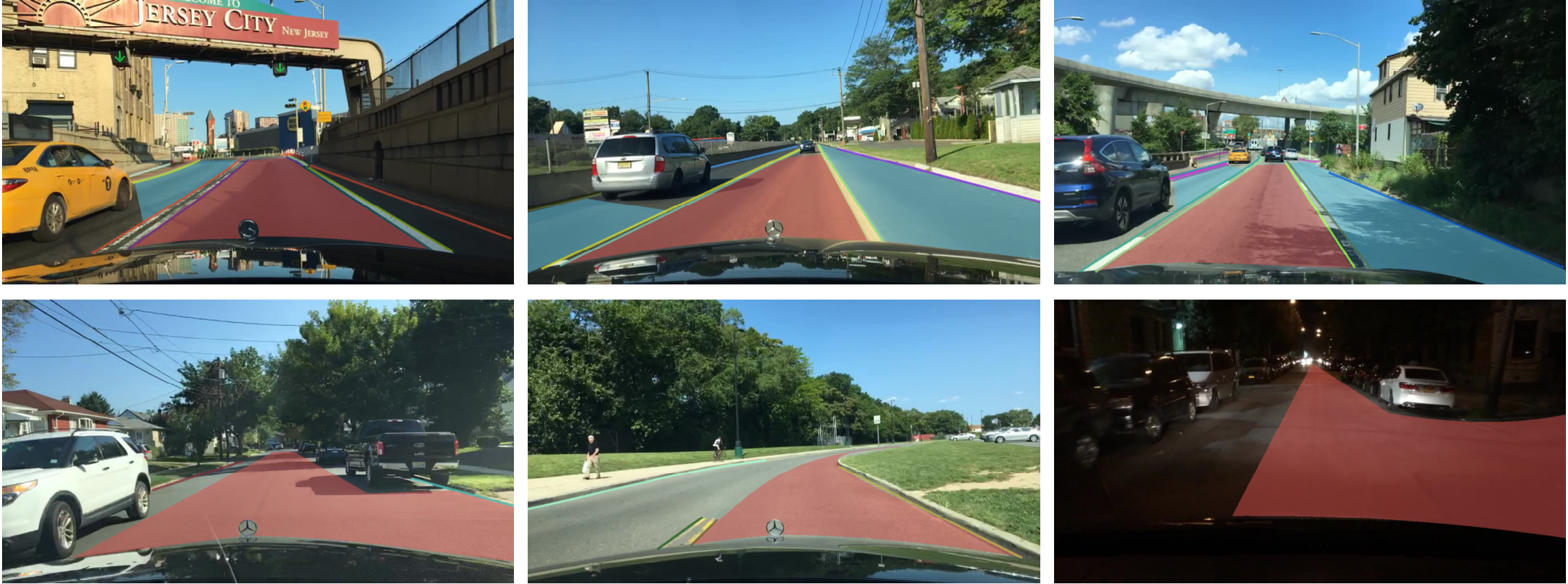
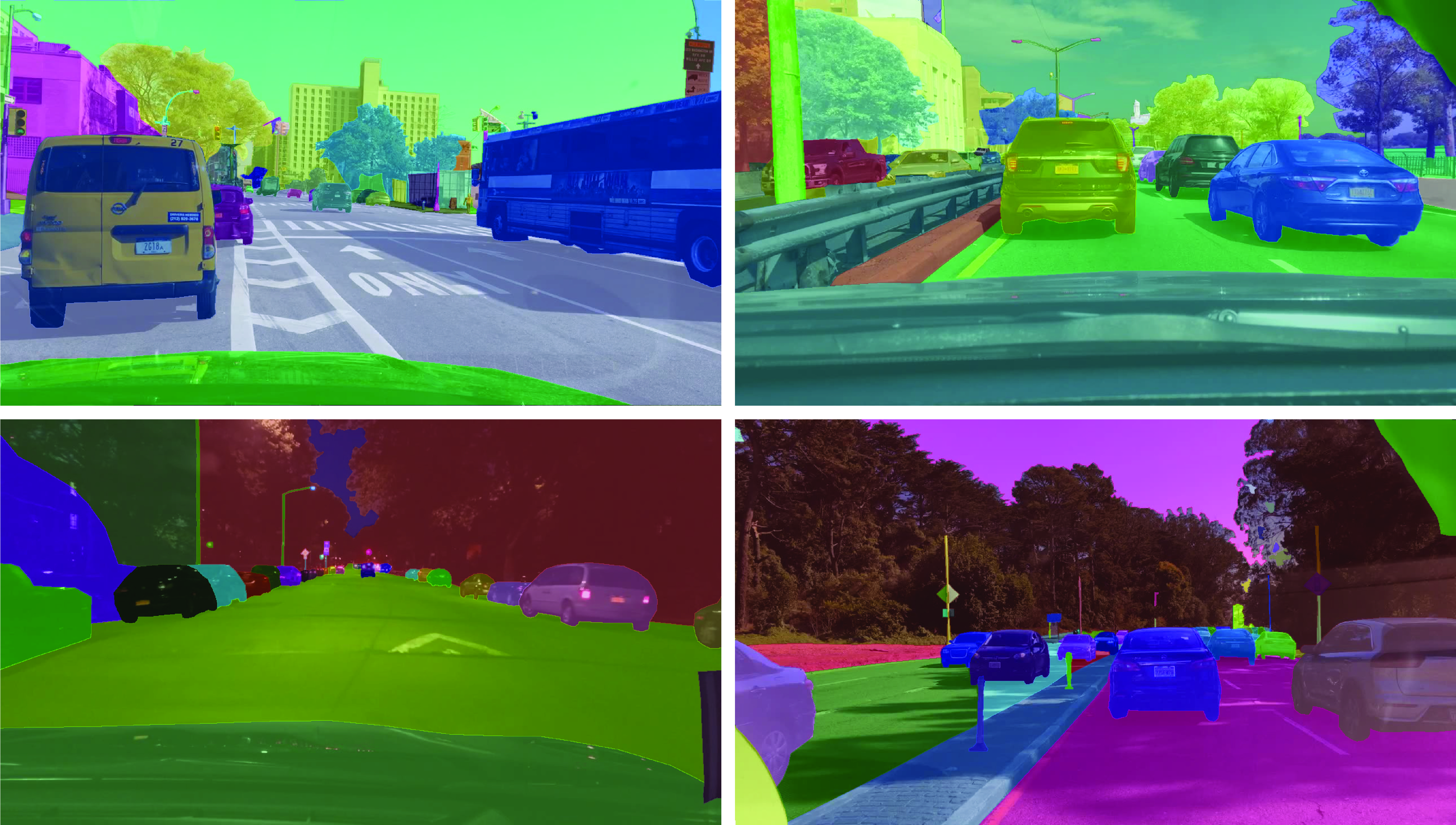
Robots, on the other hand, are typically deployed with a fixed behavior (be it hard-coded or learned), allowing them succeed in specific settings, but leading to failure in others: experiencing a system malfunction, encountering a new terrain or environment changes such as wind, or needing to cope with a payload or other unexpected perturbations. The idea behind our latest research is that the mismatch between predicted and observed recent states should inform the robot to update its model into one that more accurately describes the current situation. Noticing our car skidding on the road, for example, informs us that our actions are having a different effect than expected, and thus allows us to plan our consequent actions accordingly (Fig. 2). In order for our robots to be successful in the real world, it is critical that they have this ability to use their past experience to quickly and flexibly adapt. To this effect, we developed a model-based meta-reinforcement learning algorithm capable of fast adaptation.

Figure 2: The driver normally makes decisions based on his/her model of the world. Suddenly encountering a slippery road, however, leads to unexpected skidding. Online adaptation of the driver’s world model based on just a few of these observations of model mismatch allows for fast recovery.

Fast Adaptation

Prior work has used (a) trial-and-error adaptation approaches (Cully et al., 2015) as well as (b) model-free meta-RL approaches (Wang et al., 2016; Finn et al., 2017) to enable agents to adapt after a handful of trials. However, our work takes this adaptation ability to the extreme. Rather than adaptation requiring a few episodes of experience under the new settings, our adaptation happens online on the scale of just a few timesteps (i.e., milliseconds): so fast that it can hardly be noticed.

We achieve this fast adaptation through the use of meta-learning (discussed below) in a model-based learning setup. In the model-based setting, rather than adapting based on the rewards that are achieved during rollouts, data for updating the model is readily available at every timestep in the form of model prediction errors on recent experiences. This model-based approach enables the robot to meaningfully update the model using only a small amount of recent data.

Method Overview

Fig 3. The agent uses recent experience to fine-tune the prior model into an adapted one, which the planner then uses to perform its action selection. Note that we omit details of the update rule in this post, but we experiment with two such options in our work.

Our method follows the general formulation shown in Fig. 3 of using observations from recent data to perform adaptation of a model, and it is analogous to the overall framework of adaptive control (Sastry and Isidori, 1989; Åström and Wittenmark, 2013). The real challenge here, however, is how to successfully enable model adaptation when the models are complex, nonlinear, high-capacity function approximators (i.e., neural networks). Naively implementing SGD on the model weights is not effective, as neural networks require much larger amounts of data in order to perform meaningful learning.

Thus, we enable fast adaptation at test time by explicitly training with this adaptation objective during (meta-)training time, as explained in the following section. Once we meta-train across data from various settings in order to get this prior model (with weights denoted as $\theta^*$) that is good at adaptation, the robot can then adapt from this $\theta^*$ at each time step (Fig. 3) by using this prior in conjunction with recent experience to fine-tune its model to the current setting at hand, thus allowing for fast online adaptation.

Meta-training:

At any given time step $t$, we are in state $s_t$, we take action $a_t$, and we end up in some resulting state $s_{t+1}$ according to the underlying dynamics function $s_{t+1} = f(s_t, a_t)$. The true dynamics are unknown to us, so we instead want to fit some learned dynamics model $\hat{s}_{t+1} = f_{\theta}(s_t, a_t)$ that makes predictions as well as possible on observed data points of the form $(s_t, a_t, s_{t+1})$. Our planner can use this estimated dynamics model in order to perform action selection.

Assuming that any detail or setting could have changed at any time step along the rollout, we consider temporally-close time steps as being able to inform us about the “task” details of our current situation: operating in different parts of the state space, enduring disturbances, attempting new goals/reward, experiencing a system malfunction, etc. Thus, in order for our model to be the most useful for planning, we want to first update it using our recently observed data.

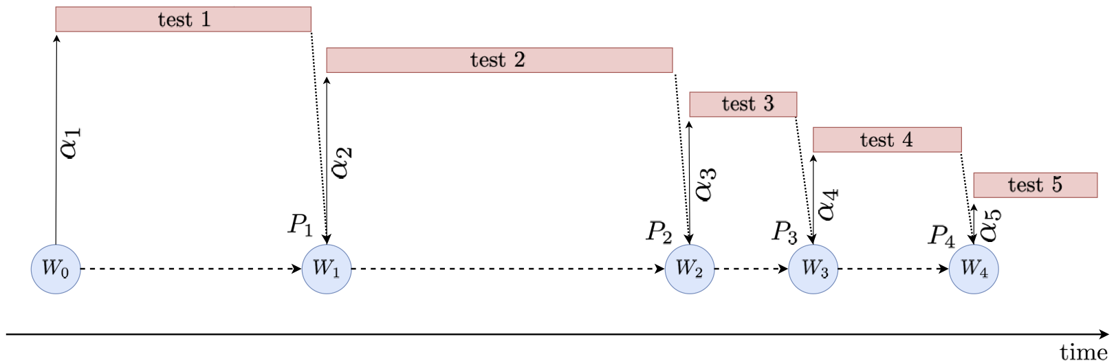
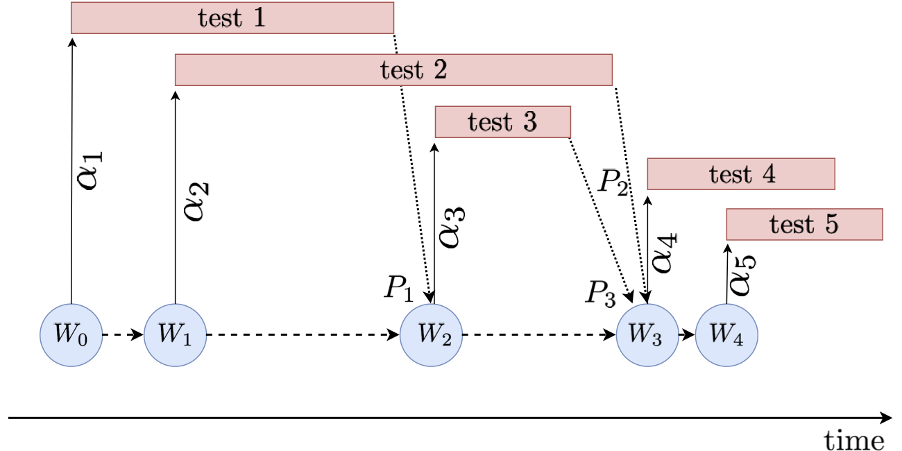
At training time (Fig. 4), what this amounts to is selecting a consecutive sequence of (M+K) data points, using the first M to update our model weights from $\theta$ to $\theta’$, and then optimizing for this new $\theta’$ to be good at predicting the state transitions for the next K time steps. This newly formulated loss function represents prediction error on the future K points, after adapting the weights using information from the past K points:

$$L = \sum_{\text{tasks}} \| f_{\theta’}(s, a) - s’ \| ^ 2 |_{\text{data}_K}$$

where

$$\theta’ = u(\theta, \text{data}_M)$$

In other words, $\theta$ does not need to result in good dynamics predictions. Instead, $\theta$ needs to be such that it can use task-specific (i.e. recent) data points to quickly adapt itself into new weights that do result in good dynamics predictions. See the MAML blog post for more intuition on this formulation.

Fig 4. Meta-training procedure for obtaining a $\theta$ such that the adaptation of $\theta$ using the past $M$ timesteps of experience produces a model that performs well for the future $K$ timesteps.

Simulation Experiments

We conducted experiments on simulated robotic systems to test the ability of our method to adapt to sudden changes in the environment, as well as to generalize beyond the training environments. Note that we meta-trained all agents on some distribution of tasks/environments (see paper for details), but we then evaluated their adaptation ability on unseen and changing environments at test time. Figure 5 shows a cheetah robot that was trained on piers of varying random buoyancy, and then tested on a pier with sections of varying buoyancy in the water. This environment demonstrates the need for not only adaptation, but for fast/online adaptation. Figure 6 also demonstrates the need for online adaptation by showing an ant robot that was trained with different crippled legs, but tested on an unseen leg failure occurring part-way through a rollout. In these qualitative results below, we compare our gradient-based adaptive learner (‘GrBAL’) to a standard model-based learner (‘MB’) that was trained on the same variation of training tasks but has no explicit mechanism for adaptation.

Fig 5. Cheetah: Both methods are trained on piers of varying buoyancy. Ours is able to perform fast online adaptation at run-time to cope with changing buoyancy over the course of a new pier.

Fig 6. Ant: Both methods are trained on different joints being crippled. Ours is able to use its recent experiences to adapt its knowledge and cope with an unexpected and new malfunction in the form of a crippled leg (for a leg that was never seen as crippled during training).

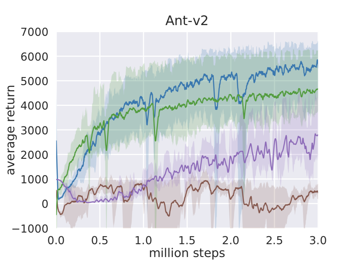
The fast adaptation capabilities of this model-based meta-RL method allow our simulated robotic systems to attain substantial improvement in performance and/or sample efficiency over prior state-of-the-art methods, as well as over ablations of this method with the choice of yes/no online adaptation, yes/no meta-training, and yes/no dynamics model. Please refer to our paper for these quantitative comparisons.

Hardware Experiments

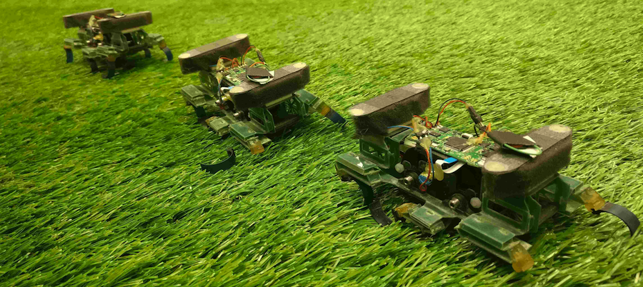
Fig 7. Our real dynamic legged millirobot, on which we successfully employ our model-based meta-reinforcement learning algorithm to enable online adaptation to disturbances and new settings such as traversing a slippery slope, accommodating payloads, accounting for pose miscalibration errors, and adjusting to a missing leg.

To highlight not only the sample efficiency of our meta reinforcement learning approach, but also the importance of fast online adaptation in the real world, we demonstrate our approach on a real dynamic legged millirobot (see Fig 7). This small 6-legged robot presents a modeling and control challenge in the form of highly stochastic and dynamic movement. This robot is an excellent candidate for online adaptation for many reasons: the rapid manufacturing techniques and numerous custom-design steps used to construct this robot make it impossible to reproduce the same dynamics each time, its linkages and other body parts deteriorate over time, and it moves very quickly and dynamically as a function of its terrain.

We meta-train this legged robot on various terrains, and we then test the agent’s learned ability to adapt online to new tasks (at run-time) including a missing leg, novel slippery terrains and slopes, miscalibration or errors in pose estimation, and new payloads to be pulled. Our hardware experiments compare our method to (a) standard model-based learning (‘MB’), with neither adaptation nor meta-learning, and well as (b) a dynamic evaluation (‘MB+DE’) comparison having adaptation, but performing the adaptation from a non-meta-learned prior. These results (Fig. 8-10) show the need for not only adaptation, but adaptation from an explicitly meta-learned prior.

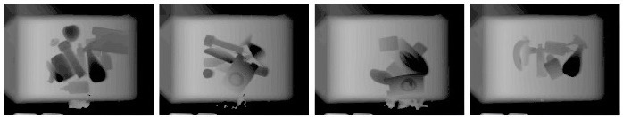
Fig 8. Missing leg.

Fig 9. Payload.

Fig 10. Miscalibrated Pose.

By effectively adapting online, our method prevents drift from a missing leg, prevents sliding sideways down a slope, accounts for pose miscalibration errors, and adjusts to pulling payloads. Note that these tasks/environments share enough commonalities with the locomotion behaviors learned during the meta-training phase such that it would be useful to draw from that prior knowledge (rather than learn from scratch), but they are different enough that they do require effective online adaptation for success.

Fig 11. The ability to draw from prior knowledge as well as to learn from recent knowledge enables GrBAL (ours) to clearly outperform both MB and MB+DE when tested on environments that (1) require online adaptation and/or (2) were never seen during training.

Future Directions

This work enables online adaptation of high-capacity neural network dynamics models, through the use of meta-learning. By allowing local fine-tuning of a model starting from a meta-learned prior, we preclude the need for an accurate global model, as well as allow for fast adaptation to new situations such as unexpected environmental changes. Although we showed results of adaptation on various tasks in both simulation and hardware, there remain numerous relevant avenues for improvement.

First, although this setup of always fine-tuning from our pre-trained prior can be powerful, one limitation of this approach is that even numerous times of seeing a new setting would result in the same performance as the 1st time of seeing it. In this follow-up work, we take steps to address precisely this issue of improving over time, while simultaneously not forgetting older skills as a consequence of experiencing new ones.

Another area for improvement includes formulating conditions or an analysis of the capabilities and limitations of this adaptation: what can or cannot be adapted to, given the knowledge contained in the prior? For example, consider two humans learning to ride a bicycle who suddenly experience a slippery road. Assume that neither of them have ridden a bike before, so they have never fallen off a bike before. Human A might fall, break their wrist, and require months of physical therapy. Human B, on the other hand, might draw from his/her prior knowledge of martial arts and thus implement a good “falling” procedure (i.e., roll onto your back instead of trying to break a fall with the wrist). This is a case when both humans are trying to execute a new task, but other experiences from their prior knowledge significantly affect the result of their adaptation attempt. Thus, having some mechanism for understanding limitations of adaptation, under the existing prior, would be interesting.

We would like to thank Sergey Levine and Chelsea Finn for their feedback during the preparation of this blog post. We would also like to thank our co-authors Simin Liu, Ronald Fearing, and Pieter Abbeel. This post is based on the following paper:

• Learning to Adapt in Dynamic, Real-World Environments Through Meta-Reinforcement Learning
  A Nagabandi*, I Clavera*, S Liu, R Fearing, P Abbeel, S Levine, C Finn
  International Conference on Learning Representations (ICLR) 2019
  Arxiv, Code, Project Page

This article was initially published on the BAIR blog, and appears here with the authors’ permission.

By Annie Xie

In many animals, tool-use skills emerge from a combination of observational learning and experimentation. For example, by watching one another, chimpanzees can learn how to use twigs to “fish” for insects. Similarly, capuchin monkeys demonstrate the ability to wield sticks as sweeping tools to pull food closer to themselves. While one might wonder whether these are just illustrations of “monkey see, monkey do,” we believe these tool-use abilities indicate a greater level of intelligence.

Left: A chimpanzee fishing for termites. Right: A gorilla using a stick to gather herbs. (source)

The question our new work explores is: can we enable robots to use tools in the same way — through observation and experimentation?

A requisite for performing complex multi-object manipulation tasks, such as those involved in tool use, is an understanding of physical cause-and-effect relationships. Therefore, the ability to predict how one object might interact with another is crucial. Our prior work has investigated how visual predictive models of cause-and-effect can be learned from unsupervised robot interaction with the world. After learning such a model, the robot can plan to accomplish a diverse set of simple tasks, including cloth folding and object arrangement. However, if we consider the more complex interactions that occur in tool-use tasks, such as how a broom can sweep dirt into a dustpan, undirected experimentation isn’t enough.

Hence, taking inspiration from how animals learn, we designed an algorithm that allows robots to learn tool-use skills through a similar paradigm of imitation and interaction. In particular, we show that, with a mix of demonstration data and unsupervised experience, a robot can use novel objects as tools and even improvise tools in the absence of traditional ones. Further, depending on the demands of the task, our method demonstrates the ability to decide whether to use the provided tools. In this post, we will describe how this works.

Read More

By Frederik Ebert and Stephen Tian

Guiding our fingers while typing, enabling us to nimbly strike a matchstick, and inserting a key in a keyhole all rely on our sense of touch. It has been shown that the sense of touch is very important for dexterous manipulation in humans. Similarly, for many robotic manipulation tasks, vision alone may not be sufficient – often, it may be difficult to resolve subtle details such as the exact position of an edge, shear forces or surface textures at points of contact, and robotic arms and fingers can block the line of sight between a camera and its quarry. Augmenting robots with this crucial sense, however, remains a challenging task.

Our goal is to provide a framework for learning how to perform tactile servoing, which means precisely relocating an object based on tactile information. To provide our robot with tactile feedback, we utilize a custom-built tactile sensor, based on similar principles as the GelSight sensor developed at MIT. The sensor is composed of a deformable, elastomer-based gel, backlit by three colored LEDs, and provides high-resolution RGB images of contact at the gel surface. Compared to other sensors, this tactile sensor sensor naturally provides geometric information in the form of rich visual information from which attributes such as force can be inferred. Previous work using similar sensors has leveraged the this kind of tactile sensor on tasks such as learning how to grasp, improving success rates when grasping a variety of objects.

Below is the real time raw sensor output as a marker cap is rolled along the gel surface:

Hardware Setup & Task Definition

For our experiments, we use a modified 3-axis CNC router with a tactile sensor mounted face-down on the end effector of the machine. The robot moves by changing the X, Y, and Z position of the sensor relative to its working stage, driving each axis with a separate stepper motor. Because of the precise control of these motors, our setup can achieve a resolution of roughly 0.04mm, helpful for careful movements in fine manipulation tasks.

The robot setup, prepared for the die rolling task is described below. The tactile sensor is mounted on the end effector at the top left of the image, facing downwards.

We demonstrate our method through three representative manipulation tasks:

1. Ball repositioning task: The robot moves a small metal ball bearing to a target location on the sensor surface. This task can be difficult because coarse control will often apply too much force on the ball bearing, causing it to slip and shoot away from the sensor with any movement.

2. Analog stick deflection task: When playing video games, we often rely solely on our sense of touch to manipulate an analog stick on a game controller. This task is of particular interest because deflecting the analog stick often requires an intentional break and return of contact, creating a partial observability situation.

3. Die rolling task: In this task, the robot rolls a 20-sided die from one face to another. In this task the risk of the object slipping out under the sensor is even greater, thus making the task the hardest of the three. An advantage of this task is that it additionally provides an intuitive success metric – when the robot has finished manipulation, is the correct number showing face up?

From left to right: The ball repositioning, analog stick, and die rolling tasks.

Each of these control tasks are specified in terms of goal images directly in tactile space; that is, the robot aims to manipulate the objects so that they produce a particular imprint upon the gel surface. These goal tactile images can be more informative and natural to specify than, say, a 3D-pose specification for an object or desired force vector.

Deep Tactile Model-Predictive Control

How can we utilize our high-dimensional sensory information to accomplish these control tasks? All three manipulation tasks can be solved using the same model-based reinforcement learning algorithm, which we call tactile model-predictive control (tactile MPC), built on top of visual foresight. It is important to note that we can use the same set of hyperparameters for each task, eliminating manual hyperparameter tuning.

A summary of deep tactile model predictive control.

The tactile MPC algorithm works by training an action-conditioned visual dynamics or video-prediction model on autonomously collected data. This model learns from raw sensory data, such as image pixels, and is able to directly make predictions of future images taking as input future hypothetical actions taken by the robot and starting tactile images we call context frames. No other information, such as the absolute position of the end effector, is specified.

Video-prediction model architecture.

In tactile MPC, as shown in the figure above, at test time, a large number of action sequences, 200 in this case, are sampled and the resulting hypothetical trajectories are predicted by the model. The trajectory which is predicted to most closely reach the goal is selected, and the first action in this sequence is taken in the real world by the robot. To allow for recovery in case of small errors in the model, trajectories the planning procedure is repeated at every step.

This control scheme has previously been applied and found success at enabling robots to lift and rearrange objects, even generalizing to previously unseen objects. If you’re interested in reading more about this, details are available in the paper.

To train the video-prediction model, we need to collect diverse data that will allow the robot to generalize to tactile states that it has not seen before. While we could sit at the keyboard and tell the robot how to move for every step of each trajectory, it would be much nicer if we could give the robot a general idea of how to collect the data, and allow it to do its thing while we catch up on homework or sleep. With a few simple reset mechanisms ensuring that things on the stage do not get out of hand over the course of data collection, we are able to collect data in a fully self-supervised manner, by collecting trajectories based on randomized action sequences. During these trajectories, the robot records tactile images from the sensor as well as the randomized actions it takes at each step. Each task required about 36 hours, in wall clock time, of data collection to train the respective predictive model, with no human supervision necessary.

Randomized data collection for the analog stick task (video sped up).

For each of the three tasks, we present representative examples of plans and rollouts:

Ball rolling task – The robot rolls the ball along the target trajectory.

Analog stick task – To reach the target goal image, the robot breaks and re-establishes contact with the object.

Die task – The robot rolls the die from the starting face labeled 20 (as seen in the prediction frames with red borders, which indicate context frames fed into the video-prediction model) to the one labeled 2.

As can be seen in these example rollouts, using the same framework and model settings, tactile MPC is able to perform a variety of manipulation tasks.

What’s Next?

We have shown a touch-based control method, tactile MPC, based on learning forward predictive models for high resolution tactile sensors, which is able to reposition objects based on user provided goals. The use of this combination of algorithms and sensors for control seems promising, and more difficult tasks may be within reach with the use of combined vision and touch sensing. However, our control horizon remains relatively short, in the tens of timesteps, which may not be sufficient for more complex manipulation tasks that we would hope to achieve in the future. In addition substantial improvements are needed on methods for specifying goals to enable more complex tasks such as general purpose object positioning or assembly.

This blog post is based on the following paper which will be presented at International Conference on Robotics and Automation 2019:

• Manipulation by Feel: Touch-Based Control with Deep Predictive Models
• Stephen Tian*, Frederik Ebert*, Dinesh Jayaraman, Mayur Mudigonda, Chelsea Finn, Roberto Calandra, Sergey Levine
• Paper link, video link

We would like to thank Sergey Levine, Roberto Calandra, Mayur Mudigonda, and Chelsea Finn for their valuable feedback when preparing this blog post. This article was initially published on the BAIR blog, and appears here with the authors’ permission.

By Tijana Zrnic

“Scientific research has changed the world. Now it needs to change itself. – The Economist, 2013

There has been a growing concern about the validity of scientific findings. A multitude of journals, papers and reports have recognized the ever smaller number of replicable scientific studies. In 2016, one of the giants of scientific publishing, Nature, surveyed about 1,500 researchers across many different disciplines, asking for their stand on the status of reproducibility in their area of research. One of the many takeaways to the worrisome results of this survey is the following: 90% of the respondents agreed that there is a reproducibility crisis, and the overall top answer to boosting reproducibility was “better understanding of statistics”. Indeed, many factors contributing to the explosion of irreproducible research stem from the neglect of the fact that statistics is no longer as static as it was in the first half of the 20th century, when statistical hypothesis testing came into prominence as a theoretically rigorous proposal for making valid discoveries with high confidence.

When science first saw the rise of statistical testing, the basic idea was the following: you put forward competing hypotheses about the world, then you collect some data, and finally you use these data to validate your hypotheses. Typically, one was in a situation where they could iterate this three-step process only a few times; data was scarce, and the necessary computations were lengthy. Remember, this is early to mid-20th century we are talking about.

This forerunner of today’s scientific investigations would hardly recognize its own field in 2019. Nowadays, testing is much more dynamic and is performed at a scale larger than ever before. Even within a single institution, thousands of hypotheses are tested in a short time interval, older test results inspire future potential analyses, and scientific exploration oftentimes becomes a never-ending stream of individual hypothesis tests. What enabled this explosion of exploratory research is the high-throughput technologies and large amounts of data that we started seeing only recently, at least relative to the era of statistical thinking.

That said, as in any discipline with well-established and successful foundations, it is difficult to move away from classical paradigms in testing. Much of today’s large-scale investigations still uses tools and techniques which, although powerful and supported by beautiful theory, do not take into account that each test might be just a little piece of a much bigger puzzle of exploratory research. Many disciplines have yet to acquire novel methodology for testing, one that promotes valid inferences at scale and thus limits grandiose publications comprised of irreplicable mirages.

Let us analyze why classical hypothesis testing might lead to many spurious conclusions when the number of tests is large. We do so by elaborating the three main steps of a test: “hypothesize”, “collect data” and “validate”.

In the “hypothesize” step, a well-defined null hypothesis is formulated. For example, this could be “jelly beans do not cause acne”; we will use this as our running example. Notice that the null hypothesis, or simply null, is the opposite of what would be considered a discovery. In short, the null is status quo. Also at the beginning of a test, a false positive rate (FPR) is chosen. This is the maximal allowed probability of making a false discovery, typically chosen around 0.05. In the context of our running example, this means the following: if the null is true, i.e. if jelly beans do not cause acne, we will only have a 5% chance of proclaiming causation between jelly beans and acne.

In a frequentist manner, we assume that there is deterministic ground truth about the null hypothesis. That is, it is either true or not. We will refer to the null hypotheses that are true as true nulls, and to those that are false as non-nulls. In our example, if jelly beans do not cause acne, the null hypothesis is a true null. If it is a non-null, however, we would ideally like to proclaim a discovery.

The second step is calculating a p-value based on collected data. This protagonist of many controversies around statistical testing is the probability of seeing the collected data, or something even more extreme, if the null is true. In our example, this is the probability of having some observed parameter of skin condition, or something “even more unusual”, if jelly beans indeed do not cause acne. To illustrate this point, consider the plot below. Let the bell curve be the distribution of the skin parameter if jelly beans do not cause acne. Then, the p-value is the red shaded area under this curve, which is everything “right of” the observed data point. The smaller the p-value, the more unlikely it is that the observation can be explained purely by chance.

[Source]

The last step is validation. If the calculated p-value is smaller than the FPR, the null hypothesis is rejected, and a discovery is proclaimed. In our running example, if the red shaded area is less than 0.05, we say that jelly beans cause acne.

Finally, let us lift the lid on why there are so many false discoveries in large-scale testing. By construction, valid p-values are uniformly distributed on $[0,1]$¹, if the null is true. This means that, even if jelly beans do not really cause acne, there is still 0.05 probability that a discovery is falsely proclaimed. Therefore, if testing N hypotheses that are truly null and hence should not be discovered, one is almost certain to proclaim some of them as discoveries if $N$ is large. For example, if all tests are independent, around 5% of $N$ will be discovered. Already after 20 tests of true nulls, even if they are completely arbitrary, one is expected to make a false discovery!

And this is how science goes wrong.

[Source]

To recap, around 5% of the tested true null hypotheses unfortunately have to be discovered either way, simply by laws of probability. This wouldn’t really be an issue if most of the tested hypotheses were legitimate potential discoveries, i.e. non-nulls. Then, 5% of a small-ish number of true nulls would be negligible. Typically, however, this is not the case. We test loads of crazy, out-there hypotheses, which would attract a lot of attention if confirmed, and we do so simply because we can. In many areas, both observations and computational resources are abundant, so there is little incentive to stay on the “safe side”.

So, how can one make scientific discoveries without the fear of reporting too many false ones?

Controlling the False Discovery Rate

The recognition that a large number of tests leads to almost sure false discoveries has led to various formalisms for controlling their rate of appearance. One powerful proposal, which has become a de facto standard for false discovery control in multiple testing, is called the false discovery rate (FDR), defined as:

$$\text{FDR} = \mathbf{E}\left[\frac{\# \text{ false discoveries}}{\# \text{ discoveries} \vee 1}\right].$$

Controlling FDR with no additional goal is an easy task; namely, making no discoveries trivially gives FDR = 0. The implict goal behind the vast literature on FDR is discovering as many non-nulls as possible, while keeping FDR controlled under a pre-specified level $\alpha$. We collectively refer to all methods with this goal as FDR methods.

Initially, FDR methods were offline procedures. This means that they required collecting a whole batch of p-values before deciding which tests to proclaim as discoveries. The most notable example of this class is the successful Benjamini-Hochberg procedure, which has for a long time been the default of FDR methods.

However, the scale and scope of modern testing have begun to outstrip this well-recognized methodology. It is far from convenient to wait for all the p-values one wants to test, especially at institutions where testing is a never-ending process. To be more precise, we typically want to make decisions during and between our tests, in particular because this allows us to shape future analyses based on outcomes of past tests. This inspired a new line of work on FDR control, in which decisions are made online.

In online FDR control, p-values arrive one at a time, and the decision of whether or not to make a discovery is made as soon as a p-value is observed. Importantly, online FDR algorithms have enabled controlling FDR over a lifetime; even if the number of sequential tests tends to infinity, one would still have a guarantee that most of the proclaimed discoveries are indeed non-nulls.

The basic principle of online FDR control is to track and control a dynamic quantity called wealth. The wealth represents the current error budget, and is a result of all previously performed tests. In particular, if a test results in a discovery, the wealth increases, while if a discovery is not made, the wealth decreases; note that this update is completely independent of whether the test is truly null or not. When a new test starts, its FPR is chosen based on the available wealth; the bigger the wealth, the bigger the FPR, and consequently the better the chance for a discovery. In fact, this idea has a perfect analogy with testing in a broader social context. To make scientific discoveries, you are awarded an initial grant (corresponding to the target FDR level $\alpha$). This initial funding decreases with every new experiment, and, if you happen to make a scientific discovery, you are again awarded some “wealth”, which you can use toward the budget for subsequent tests. This is essentially the real-world translation of the mathematical expressions guiding online FDR algorithms.

Asynchronous Control of False Discoveries

Although online FDR control has broadened the domain of applications where false discoveries can be controlled, it has failed to account for several important aspects of modern testing.

The main observation is that large-scale testing is not only sequential, but “doubly sequential”. Tests are run in a sequential fashion, but also each test internally is comprised of a sequence of atomic executions, which typically finish at an unpredictable time. This fact makes practitioners run multiple tests that overlap in time in order to gain time efficiency, allowing tests to start and finish at random times.

For example, in clinical trials, it is common to test several different treatment variants against a common control. These trials are often called “perpetual’’, as multiple treatments are tested in parallel, and new treatments enter the testing platform at random times in an online manner. Similarly, A/B testing in industry is typically distributed across many individuals and research teams, and across time, with companies running hundreds of tests per day. This large volume of tests, as well as their complex distribution across many analysts, inevitably causes asynchrony in testing.

This circumstance is a problem for standard online FDR methodology. Namely, all existing online FDR algorithms assume tests are run synchronously, with no overlap in time; in other words, in order to determine a false positive rate for an upcoming test, online FDR methods need to know the outcomes of all previously started tests. The figure below depicts the difference between synchronous and asynchronous online testing.

For each time step $t$, $W_t$, $P_t$ and $\alpha_t$ are respectively the available wealth at the beginning of the $(t+1)$-th test, the p-value resulting from the $t$-th test, and the FPR of the $t$-th test.

Furthermore, the asynchronous nature of modern testing introduces patterns of dependence between p-values that do not conform to common assumptions. Prior work on online FDR either assumes perfect independence between p-values (overly optimistic), or arbitrary dependence between all tested p-values in the sequence (overly pessimistic). As data are commonly shared across different tests, the first assumption in clearly difficult to satisfy. In clinical trials, having a common control arm induces dependence; in A/B testing, many tests reuse data from the same shared pool, again causing dependence. On the other end, it is not natural to assume that dependence spills over the entire p-value sequence; older data and test outcomes with time become “stale,” and no longer have direct influence on newly created tests. Modern testing calls for an intermediate notion of dependence, called local dependence, one that assumes p-values that are far enough in the sequence are independent, while any two close enough are likely to depend on each other.

In a recent manuscript [1], we developed FDR methods that confront both of these difficulties of large-scale testing. Our methods control FDR in sequential settings that are arbitrarily asynchronous, and/or yield p-values that are locally dependent. Interestingly, from the point of view of our analysis, both local dependence and asynchrony are solved via the same technical instrument, which we call conflict sets. More formally, each new test has a conflict set, which consists of all previously started tests whose outcome is not known (e.g. if there is asynchrony so they are still running), or is known but might have some leverage on the new test (e.g. if there is dependence). We show that computing the FPR of a new test while assuming “unfavorable” outcomes of the conflicting tests is the right approach to guaranteeing FDR control (we call this the principle of pessimism).

It is worth pointing out that FDR control under conflict sets has to be more conservative by construction; to account for dependence between tests, as well as the uncertainty about the tests in progress, the FPRs have to be chosen appropriately smaller. That said, our methods are a strict generalization of prior work on online FDR; they interpolate between standard online FDR algorithms, when the conflict sets are empty, and the Bonferroni correction (also known as alpha-spending), when the conflict sets are arbitrarily large. The latter controls the familywise error rate, which is a more stringent error metric than FDR, under any assumption on how tests relate. This interpolation has introduced the possibility of a tradeoff between the consideration of overall rate of discovery per unit of real time, and consideration of the complexity of careful coordination required to minimize dependence and asynchrony.

Summary

The replicability of hypothesis tests is largely in crisis, as the scale of modern applications has long outstripped classical testing methodology which is still in use. Moreover, prior efforts toward remedying this problem have neglected the fact that testing is massively asynchronous, and hence the existing solutions for boosting reproducibility have not been suitable for many common large-scale testing schemes. Motivated by this observation, we developed methods that control the false discovery rate in complex asynchronous scenarios, allowing statisticians to perform hypothesis tests with a small fraction of false discoveries, and with minimal explicit coordination between tests.

This article was initially published on the BAIR blog, and appears here with the authors’ permission.

References

[1] Zrnic, T., Ramdas, A., & Jordan, M. I. (2018). Asynchronous Online Testing of Multiple Hypotheses. arXiv preprint arXiv:1812.05068.

By Rohin Shah and Dmitrii Krasheninnikov

It would be great if we could all have household robots do our chores for us. Chores are tasks that we want done to make our houses cater more to our preferences; they are a way in which we want our house to be different from the way it currently is. However, most “different” states are not very desirable:

Surely our robot wouldn’t be so dumb as to go around breaking stuff when we ask it to clean our house? Unfortunately, AI systems trained with reinforcement learning only optimize features specified in the reward function and are indifferent to anything we might’ve inadvertently left out. Generally, it is easy to get the reward wrong by forgetting to include preferences for things that should stay the same, since we are so used to having these preferences satisfied, and there are so many of them. Consider the room below, and imagine that we want a robot waiter that serves people at the dining table efficiently. We might implement this using a reward function that provides 1 reward whenever the robot serves a dish, and use discounting so that the robot is incentivized to be efficient. What could go wrong with such a reward function? How would we need to modify the reward function to take this into account? Take a minute to think about it.

Here’s an incomplete list we came up with:

• The robot might track dirt and oil onto the pristine furniture while serving food, even if it could clean itself up, because there’s no reason to clean but there is a reason to hurry.
• In its hurry to deliver dishes, the robot might knock over the cabinet of wine bottles, or slide plates to people and knock over the glasses.
• In case of an emergency, such as the electricity going out, we don’t want the robot to keep trying to serve dishes – it should at least be out of the way, if not trying to help us.
• The robot may serve empty or incomplete dishes, dishes that no one at the table wants, or even split apart dishes into smaller dishes so there are more of them.

Note that we’re not talking about problems with robustness and distributional shift: while those problems are worth tackling, the point is that even if we achieve robustness, the simple reward function still incentivizes the above unwanted behaviors.

It’s common to hear the informal solution that the robot should try to minimize its impact on the environment, while still accomplishing the task. This could potentially allow us to avoid the first three problems above, though the last one still remains as an example of specification gaming. This idea leads to impact measures that attempt to quantify the “impact” that an agent has, typically by looking at the difference between what actually happened and what would have happened had the robot done nothing. However, this also penalizes things we want the robot to do. For example, if we ask our robot to get us coffee, it might buy coffee rather than making coffee itself, because that would have “impact” on the water, the coffee maker, etc. Ultimately, we’d like to only prevent negative impacts, which means that we need our AI to have a better idea of what the right reward function is.

Our key insight is that while it might be hard for humans to make their preferences explicit, some preferences are implicit in the way the world looks: the world state is a result of humans having acted to optimize their preferences. This explains why we often want the robot to by default “do nothing” – if we have already optimized the world state for our preferences, then most ways of changing it will be bad, and so doing nothing will often (though not always) be one of the better options available to the robot.

Since the world state is a result of optimization for human preferences, we should be able to use that state to infer what humans care about. For example, we surely don’t want dirty floors in our pristine room; otherwise we would have done that ourselves. We also can’t be indifferent to dirty floors, because then at some point we would have walked around the room with dirty shoes and gotten a dirty floor. The only explanation is that we want the floor to be clean.

A simple setting

Let’s see if we can apply this insight in the simplest possible setting: gridworlds with a small number of states, a small number of actions, a known dynamics model (i.e. a model of “how the world works”), but an incorrect reward function. This is a simple enough setting that our robot understands all of the consequences of its actions. Nevertheless, the problem remains: while the robot understands what will happen, it still cannot distinguish good consequences from bad ones, since its reward function is incorrect. In these simple environments, it’s easy to figure out what the correct reward function is, but this is infeasible in a real, complex environment.

For example, consider the room to the right, where Alice asks her robot to navigate to the purple door. If we were to encode this as a reward function that only rewards the robot while it is at the purple door, the robot would take the shortest path to the purple door, knocking over and breaking the vase – since no one said it shouldn’t do that. The robot is perfectly aware that its plan causes it to break the vase, but by default it doesn’t realize that it shouldn’t break the vase.

In this environment, does it help us to realize that Alice was optimizing the state of the room for her preferences? Well, if Alice didn’t care about whether the vase was broken, she would have probably broken it some time in the past. If she wanted the vase broken, she definitely would have broken it some time in the past. So the only consistent explanation is that Alice cared about the vase being intact, as illustrated in the gif below.

While this example has the robot infer that it shouldn’t take the action of breaking a vase, the robot can also infer goals that it should actively pursue. For example, if the robot observes a basket of apples near an apple tree, it can reasonably infer that Alice wants to harvest apples, since the apples didn’t walk into the basket themselves – Alice must have put effort into picking the apples and placing them in the basket.

Reward Learning by Simulating the Past

We formalize this idea by considering an MDP in which our robot observes the initial state $s_0$ at deployment, and assumes that it is the result of a human optimizing some unknown reward for $T$ timesteps.

Before we get to our actual algorithm, consider a completely intractable algorithm that should do well: for each possible reward function, simulate the trajectories that Alice would take if she had that reward, and see if the resulting states are compatible with $s_0$. This set of compatible reward functions give the candidates for Alice’s reward function. This is the algorithm that we implicitly use in the gif above.

Intuitively, this works because:

• Anything that requires effort on Alice’s part (e.g. keeping a vase intact) will not happen for the vast majority of reward functions, and will force the reward functions to incentivize that behavior (e.g. by rewarding intact vases).
• Anything that does not require effort on Alice’s part (e.g. a vase becoming dusty) will happen for most reward functions, and so the inferred reward functions need not incentivize that behavior (e.g. there’s no particular value on dusty/clean vases).

Another way to think of it is that we can consider all possible past trajectories that are compatible with $s_0$, infer the reward function that makes those trajectories most likely, and keep those reward functions as plausible candidates, weighted by the number of past trajectories they explain. Such an algorithm should work for similar reasons. Phrased this way, it sounds like we want to use inverse reinforcement learning to infer rewards for every possible past trajectory, and aggregate the results. This is still intractable, but it turns out we can take this insight and turn it into a tractable algorithm.

We follow Maximum Causal Entropy Inverse Reinforcement Learning (MCEIRL), a commonly used algorithm for small MDPs. In this framework, we know the action space and dynamics of the MDP, as well as a set of good features of the state, and the reward is assumed to be linear in these features. In addition, the human is modelled as Boltzmann-rational: Alice’s probability of taking a particular action from a given state is assumed to be proportional to the exponent of the state-action value function Q, computed using soft value iteration. Given these assumptions, we can calculate $p(\tau \mid \theta_A)$, the distribution over the possible trajectories $\tau = s_{-T} a_{-T} \dots s_{-1} a_{-1} s_0$ under the assumption that Alice’s reward was $\theta_A$. MCEIRL then finds the $\theta_A$ that maximizes the probability of a set of trajectories $\{\tau_i\}$.

Rather than considering all possible trajectories and running MCEIRL on all of them to maximize each of their probabilities individually, we instead maximize the probability of the evidence that we see: the single state $s_0$. To get a distribution over $s_0$, we marginalize out the human’s behavior prior to the robot’s initialization:

$$P(s_0 \mid \theta_A) = \sum\limits_{s_{-T}a_{-T} \dots s_{-1}a_{-1}} P(s_{-T} a_{-T} \dots s_{-1} a_{-1} s_0 \mid \theta_A)$$

We then find a reward $\theta_A$ that maximizes the likelihood above using gradient ascent, where the gradient is analytically computed using dynamic programming. We call this algorithm Reward Learning by Simulating the Past (RLSP) since it infers the unknown human reward from a single state by considering what must have happened in the past.

Using the inferred reward

While RLSP infers a reward that captures the information about human preferences contained in the initial state, it is not clear how we should use that reward. This is a challenging problem – we have two sources of information, the inferred reward from $s_0$, and the specified reward $\theta_{\text{spec}}$, and they will conflict. If Alice has a messy room, $\theta_A$ is not going to incentivize cleanliness, even though $\theta_{\text{spec}}$ might.

Ideally, we would note the scenarios under which the two rewards conflict, and ask Alice how she would like to proceed. However, in this work, to demonstrate the algorithm we use the simple heuristic of adding the two rewards, giving us a final reward $\theta_A + \lambda \theta_{\text{spec}}$, where $\lambda$ is a hyperparameter that controls the tradeoff between the rewards.

We designed a suite of simple gridworlds to showcase the properties of RLSP. The top row shows the behavior when optimizing the (incorrect) specified reward, while the bottom row shows the behavior you get when you take into account the reward inferred by RLSP. A more thorough description of each environment is given in the paper. The last environment in particular shows a limitation of our method. In a room where the vase is far away from Alice’s most probable trajectories, the only trajectories that Alice could have taken to break the vase are all very long and contribute little to the RLSP likelihood. As a result, observing the intact vase doesn’t tell the robot much about whether Alice wanted to actively avoid breaking the vase, since she wouldn’t have been likely to break it in any case.

What’s next?

Now that we have a basic algorithm that can learn the human preferences from one state, the natural next step is to scale it to realistic environments where the states cannot be enumerated, the dynamics are not known, and the reward function is not linear. This could be done by adapting existing inverse RL algorithms, similarly to how we adapted Maximum Causal Entropy IRL to the one-state setting.

The unknown dynamics setting, where we don’t know “how the world works”, is particularly challenging. Our algorithm relies heavily on the assumption that our robot knows how the world works – this is what gives it the ability to simulate what Alice “must have done” in the past. We certainly can’t learn how the world works just by observing a single state of the world, so we would have to learn a dynamics model while acting that can then be used to simulate the past (and these simulations will get better as the model gets better).

Another avenue for future work is to investigate the ways to decompose the inferred reward into $\theta_{A, \text{task}}$ which says which task Alice is performing (“go to the black door”), and $\theta_{\text{frame}}$, which captures what Alice prefers to keep unchanged (“don’t break the vase”). Given the separate $\theta_{\text{frame}}$, the robot could optimize $\theta_{\text{spec}}+\theta_{\text{frame}}$ and ignore the parts of the reward function that correspond to the task Alice is trying to perform.

Since $\theta_{\text{frame}}$ is in large part shared across many humans, we could infer it using models where multiple humans are optimizing their own unique $\theta_{H,\text{task}}$ but the same $\theta_{\text{frame}}$, or we could have one human whose task change over time. Another direction would be to assume a different structure for what Alice prefers to keep unchanged, such as constraints, and learn them separately.

You can learn more about this research by reading our paper, or by checking out our poster at ICLR 2019. The code is available here.

This article was initially published on the BAIR blog, and appears here with the authors’ permission.

By Tuomas Haarnoja, Vitchyr Pong, Kristian Hartikainen, Aurick Zhou, Murtaza Dalal, and Sergey Levine

We are announcing the release of our state-of-the-art off-policy model-free reinforcement learning algorithm, soft actor-critic (SAC). This algorithm has been developed jointly at UC Berkeley and Google Brain, and we have been using it internally for our robotics experiment. Soft actor-critic is, to our knowledge, one of the most efficient model-free algorithms available today, making it especially well-suited for real-world robotic learning. In this post, we will benchmark SAC against state-of-the-art model-free RL algorithms and showcase a spectrum of real-world robot examples, ranging from manipulation to locomotion. We also release our implementation of SAC, which is particularly designed for real-world robotic systems.

Desired Features for Deep RL for Real Robots

What makes an ideal deep RL algorithm for real-world systems? Real-world experimentation brings additional challenges, such as constant interruptions in the data stream, requirement for a low-latency inference and smooth exploration to avoid mechanical wear and tear on the robot, which set additional requirement for both the algorithm and also the implementation of the algorithm.

Regarding the algorithm, several properties are desirable:

• Sample Efficiency. Learning skills in the real world can take a substantial amount of time. Prototyping a new task takes several trials, and the total time required to learn a new skill quickly adds up. Thus good sample complexity is the first prerequisite for successful skill acquisition.
• No Sensitive Hyperparameters. In the real world, we want to avoid parameter tuning for the obvious reason. Maximum entropy RL provides a robust framework that minimizes the need for hyperparameter tuning.
• Off-Policy Learning. An algorithm is off-policy if we can reuse data collected for another task. In a typical scenario, we need to adjust parameters and shape the reward function when prototyping a new task, and use of an off-policy algorithm allows reusing the already collected data.

Soft actor-critic (SAC), described below, is an off-policy model-free deep RL algorithm that is well aligned with these requirements. In particular, we show that it is sample efficient enough to solve real-world robot tasks in only a handful of hours, robust to hyperparameters and works on a variety of simulated environments with a single set of hyperparameters.

In addition to the desired algorithmic properties, experimentation in the real-world sets additional requirements for the implementation. Our release supports many of these features that we have found crucial when learning with real robots, perhaps the most importantly:

• Asynchronous Sampling. Inference needs to be fast to minimize delay in the control loop, and we typically want to keep training during the environment resets too. Therefore, data sampling and training should run in independent threads or processes.
• Stop / Resume Training. When working with real hardware, whatever can go wrong, will go wrong. We should expect constant interruptions in the data stream.
• Action smoothing. Typical Gaussian exploration makes the actuators jitter at high frequency, potentially damaging the hardware. Thus temporally correlating the exploration is important.

Soft Actor-Critic

Soft actor-critic is based on the maximum entropy reinforcement learning framework, which considers the entropy augmented objective

$$J(\pi) = \mathbb{E}_{\pi} \left[ {\sum_{t} r(\mathbf{s}_t, \mathbf{a}_t) - \alpha \log (\pi(\mathbf{a}_t|\mathbf{s}_t))} \right],$$

where $\mathbf{s}_t$ and $\mathbf{a}_t$ are the state and the action, and the expectation is taken over the policy and the true dynamics of the system. In other words, the optimal policy not only maximizes the expected return (first summand) but also the expected entropy of itself (second summand). The trade-off between the two is controlled by the non-negative temperature parameter $\alpha$, and we can always recover the conventional, maximum expected return objective by setting $\alpha=0$. In a technical report, we show that we can view this objective as an entropy constrained maximization of the expected return, and learn the temperature parameter automatically instead of treating it as a hyperparameter.

This objective can be interpreted in several ways. We can view the entropy term as an uninformative (uniform) prior over the policy, but we can also view it as a regularizer or as an attempt to trade off between exploration (maximize entropy) and exploitation (maximize return). In our previous post, we gave a broader overview and proposed applications that are unique to maximum entropy RL, and a probabilistic view of the objective is discussed in a recent tutorial. Soft actor-critic maximizes this objective by parameterizing a Gaussian policy and a Q-function with a neural network, and optimizing them using approximate dynamic programming. We defer further details of soft actor-critic to the technical report. In this post, we will view the objective as a grounded way to derive better reinforcement learning algorithms that perform consistently and are sample efficient enough to be applicable to real-world robotic applications, and—perhaps surprisingly—can yield state-of-the-art performance under the conventional, maximum expected return objective (without entropy regularization) in simulated benchmarks.

Simulated Benchmarks

Before we jump into real-world experiments, we compare SAC on standard benchmark tasks to other popular deep RL algorithms, deep deterministic policy gradient (DDPG), twin delayed deep deterministic policy gradient (TD3), and proximal policy optimization (PPO). The figures below compare the algorithms on three challenging locomotion tasks, HalfCheetah, Ant, and Humanoid, from OpenAI Gym. The solid lines depict the total average return and the shadings correspond to the best and the worst trial over five random seeds. Indeed, soft actor-critic, which is shown in blue, achieves the best performance, and—what’s even more important for real-world applications—it performs well also in the worst case. We have included more benchmark results in the technical report.

Deep RL in the Real World

We tested soft actor-critic in the real world by solving three tasks from scratch without relying on simulation or demonstrations. Our first real-world task involves the Minitaur robot, a small-scale quadruped with eight direct-drive actuators. The action space consists of the swing angle and the extension of each leg, which are then mapped to desired motor positions and tracked with a PD controller. The observations include the motor angles as well as roll and pitch angles and angular velocities of the base. This learning task presents substantial challenges for real-world reinforcement learning. The robot is underactuated, and must therefore delicately balance contact forces on the legs to make forward progress. An untrained policy can lose balance and fall, and too many falls will eventually damage the robot, making sample-efficient learning essentially. The video below illustrates the learned skill. Although we trained our policy only on flat terrain, we then tested it on varied terrains and obstacles. Because soft actor-critic learns robust policies, due to entropy maximization at training time, the policy can readily generalize to these perturbations without any additional learning.

The Minitaur robot (Google Brain, Tuomas Haarnoja, Sehoon Ha, Jie Tan, and Sergey Levine).

Our second real-world robotic task involves training a 3-finger dexterous robotic hand to manipulate an object. The hand is based on the Dynamixel Claw hand, discussed in another post. This hand has 9 DoFs, each controlled by a Dynamixel servo-motor. The policy controls the hand by sending target joint angle positions for the on-board PID controller. The manipulation task requires the hand to rotate a “valve’‘-like object as shown in the animation below. In order to perceive the valve, the robot must use raw RGB images shown in the inset at the bottom right. The robot must rotate the valve so that the colored peg faces the right (see video below). The initial position of the valve is reset uniformly at random for each episode, forcing the policy to learn to use the raw RGB images to perceive the current valve orientation. A small motor is attached to the valve to automate resets and to provide the ground truth position for the determination of the reward function. The position of this motor is not provided to the policy. This task is exceptionally challenging due to both the perception challenges and the need to control a hand with 9 degrees of freedom.

Rotating a valve with a dexterous hand, learned directly from raw pixels (UC Berkeley, Kristian Hartikainen, Vikash Kumar, Henry Zhu, Abhishek Gupta, Tuomas Haarnoja, and Sergey Levine).

In the final task, we trained a 7-DoF Sawyer robot to stack Lego blocks. The policy receives the joint positions and velocities, as well as end-effector force as an input and outputs torque commands to each of the seven joints. The biggest challenge is to accurately align the studs before exerting a downward force to overcome the friction between them.

Stacking Legos with Sawyer (UC Berkeley, Aurick Zhou, Tuomas Haarnoja, and Sergey Levine).

Soft actor-critic solves all of these tasks quickly: the Minitaur locomotion and the block-stacking tasks both take 2 hours, and the valve-turning task from image observations takes 20 hours. We also learned a policy for the valve-turning task without images by providing the actual valve position as an observation to the policy. Soft actor-critic can learn this easier version of the valve task in 3 hours. For comparison, prior work has used PPO to learn the same task without images in 7.4 hours.

Conclusion

Soft actor-critic is a step towards feasible deep RL with real-world robots. Work still needs to be done to scale up these methods to more challenging tasks, but we believe we are getting closer to the critical point where deep RL can become a practical solution for robotic tasks. Meanwhile, you can connect your robot to our toolbox and get learning started!

Acknowledgements

We would like to thank the amazing teams at Google Brain and UC Berkeley—specifically Pieter Abbeel, Abhishek Gupta, Sehoon Ha, Vikash Kumar, Sergey Levine, Jie Tan, George Tucker, Vincent Vanhoucke, Henry Zhu—who contributed to the development of the algorithm, spent long days running experiments, and provided the support and resources that made the project possible.

This article was initially published on the BAIR blog, and appears here with the authors’ permission.

Links:

• Project website
• Technical description of SAC
• softlearning (our robot learning toolbox, including a SAC implementation in Tensorflow)
• rlkit (another SAC implementation from UC Berkeley in PyTorch)

By Chelsea Finn∗, Frederik Ebert∗, Sudeep Dasari, Annie Xie, Alex Lee, and Sergey Levine

With very little explicit supervision and feedback, humans are able to learn a wide range of motor skills by simply interacting with and observing the world through their senses. While there has been significant progress towards building machines that can learn complex skills and learn based on raw sensory information such as image pixels, acquiring large and diverse repertoires of general skills remains an open challenge. Our goal is to build a generalist: a robot that can perform many different tasks, like arranging objects, picking up toys, and folding towels, and can do so with many different objects in the real world without re-learning for each object or task.

While these basic motor skills are much simpler and less impressive than mastering Chess or even using a spatula, we think that being able to achieve such generality with a single model is a fundamental aspect of intelligence.

The key to acquiring generality is diversity. If you deploy a learning algorithm in a narrow, closed-world environment, the agent will recover skills that are successful only in a narrow range of settings. That’s why an algorithm trained to play Breakout will struggle when anything about the images or the game changes. Indeed, the success of image classifiers relies on large, diverse datasets like ImageNet. However, having a robot autonomously learn from large and diverse datasets is quite challenging. While collecting diverse sensory data is relatively straightforward, it is simply not practical for a person to annotate all of the robot’s experiences. It is more scalable to collect completely unlabeled experiences. Then, given only sensory data, akin to what humans have, what can you learn? With raw sensory data there is no notion of progress, reward, or success. Unlike games like Breakout, the real world doesn’t give us a score or extra lives.

We have developed an algorithm that can learn a general-purpose predictive model using unlabeled sensory experiences, and then use this single model to perform a wide range of tasks.

With a single model, our approach can perform a wide range of tasks, including lifting objects, folding shorts, placing an apple onto a plate, rearranging objects, and covering a fork with a towel.

In this post, we will describe how this works. We will discuss how we can learn based on only raw sensory interaction data (i.e. image pixels, without requiring object detectors or hand-engineered perception components). We will show how we can use what was learned to accomplish many different user-specified tasks. And, we will demonstrate how this approach can control a real robot from raw pixels, performing tasks and interacting with objects that the robot has never seen before.

Read More

By Esther Rolf∗, David Fridovich-Keil∗, and Max Simchowitz

In many tasks in machine learning, it is common to want to answer questions given fixed, pre-collected datasets. In some applications, however, we are not given data a priori; instead, we must collect the data we require to answer the questions of interest.

This situation arises, for example, in environmental contaminant monitoring and census-style surveys. Collecting the data ourselves allows us to focus our attention on just the most relevant sources of information. However, determining which of these sources of information will yield useful measurements can be difficult. Furthermore, when data is collected by a physical agent (e.g. robot, satellite, human, etc.) we must plan our measurements so as to reduce costs associated with the motion of the agent over time. We call this abstract problem embodied adaptive sensing.

We introduce a new approach to the embodied adaptive sensing problem, in which a robot must traverse its environment to identify locations or items of interest. Adaptive sensing encompasses many well-studied problems in robotics, including the rapid identification of accidental contamination leaks and radioactive sources, and finding individuals in search and rescue missions. In such settings, it is often critical to devise a sensing trajectory that returns a correct solution as quickly as possible.

Read More

By Daniel Seita, Jeff Mahler, Mike Danielczuk, Matthew Matl, and Ken Goldberg

This post explores two independent innovations and the potential for combining them in robotics. Two years before the AlexNet results on ImageNet were released in 2012, Microsoft rolled out the Kinect for the X-Box. This class of low-cost depth sensors emerged just as Deep Learning boosted Artificial Intelligence by accelerating performance of hyper-parametric function approximators leading to surprising advances in image classification, speech recognition, and language translation.

Top left: image of a 3D cube. Top right: example depth image, with darker points representing areas closer to the camera (source: Wikipedia). Next two rows: examples of depth and RGB image pairs for grasping objects in a bin. Last two rows: similar examples for bed-making.

Today, Deep Learning is also showing promise for end-to-end learning of playing video games and performing robotic manipulation tasks.

For robot perception, convolutional neural networks (CNNs), such as VGG or ResNet, with three RGB color channels have become standard. For robotics and computer vision tasks, it is common to borrow one of these architectures (along with pre-trained weights) and then to perform transfer learning or fine-tuning on task-specific data. But in some tasks, knowing the colors in an image may provide only limited benefits. Consider training a robot to grasp novel, previously unseen objects. It may be more important to understand the geometry of the environment rather than colors and textures. The physical process of manipulation — controlling one or more objects by applying forces through contact — depends on object geometry, pose, and other factors which are largely color-invariant. When you manipulate a pen with your hand, for instance, you can often move it seamlessly without looking at the actual pen, so long as you have a good understanding of the location and orientation of contact points. Thus, before proceeding, one might ask: does it makes sense to use color images?

There is an alternative: depth images. These are single-channel grayscale images that measure depth values from the camera, and give us invariance to the colors of objects within an image. We can also use depth to “filter” points beyond a certain distance which can remove background noise, as we demonstrate later with robot bed-making. Examples of paired depth and real images are shown above.

In this post, we consider the potential for combining depth images and deep learning in the context of three ongoing projects in the UC Berkeley AUTOLab: Dex-Net for robot grasping, segmenting objects in heaps, and robot bed-making.

Read More

By Xue Bin (Jason) Peng and Angjoo Kanazawa

Whether it’s everyday tasks like washing our hands or stunning feats of acrobatic prowess, humans are able to learn an incredible array of skills by watching other humans. With the proliferation of publicly available video data from sources like YouTube, it is now easier than ever to find video clips of whatever skills we are interested in.

Simulated characters imitating skills from YouTube videos.

A staggering 300 hours of videos are uploaded to YouTube every minute. Unfortunately, it is still very challenging for our machines to learn skills from this vast volume of visual data. Most imitation learning approaches require concise representations, such as those recorded from motion capture (mocap). But getting mocap data can be quite a hassle, often requiring heavy instrumentation. Mocap systems also tend to be restricted to indoor environments with minimal occlusion, which can limit the types of skills that can be recorded. So wouldn’t it be nice if our agents can also learn skills by watching video clips?

In this work, we present a framework for learning skills from videos (SFV). By combining state-of-the-art techniques in computer vision and reinforcement learning, our system enables simulated characters to learn a diverse repertoire of skills from video clips. Given a single monocular video of an actor performing some skill, such as a cartwheel or a backflip, our characters are able to learn policies that reproduce that skill in a physics simulation, without requiring any manual pose annotations.

Read More

In this post, we demonstrate how deep reinforcement learning (deep RL) can be used to learn how to control dexterous hands for a variety of manipulation tasks. We discuss how such methods can learn to make use of low-cost hardware, can be implemented efficiently, and how they can be complemented with techniques such as demonstrations and simulation to accelerate learning.

Why Dexterous Hands?

A majority of robots in use today use simple parallel jaw grippers as manipulators, which are sufficient for structured settings like factories. However, manipulators that are capable of performing a wide array of tasks are essential for unstructured human-centric environments like the home. Multi-fingered hands are among the most versatile manipulators, and enable a wide variety of skills we use in our everyday life such as moving objects, opening doors, typing, and painting.

Unfortunately, controlling dexterous hands is extremely difficult, which limits their use. High-end hands can also be extremely expensive, due to delicate sensing and actuation. Deep reinforcement learning offers the promise of automating complex control tasks even with cheap hardware, but many applications of deep RL use huge amounts of simulated data, making them expensive to deploy in terms of both cost and engineering effort. Humans can learn motor skills efficiently, without a simulator and millions of simulations.

We will first show that deep RL can in fact be used to learn complex manipulation behaviors by training directly in the real world, with modest computation and low-cost robotic hardware, and without any model or simulator. We then describe how learning can be further accelerated by incorporating additional sources of supervision, including demonstrations and simulation. We demonstrate learning on two separate hardware platforms: an inexpensive custom-built 3-fingered hand (the Dynamixel Claw), which costs under \$2500, and the higher-end Allegro hand, which costs about \$15,000.

Left: Dynamixel Claw. Right: Allegro Hand.

Model-free Reinforcement Learning in the Real World

Deep RL algorithms learn by trial and error, maximizing a user-specified reward function from experience. We’ll use a valve rotation task as a working example, where the hand must open a valve or faucet by rotating it 180 degrees.

Illustration of valve rotation task.

The reward function simply consists of the negative distance between the current and desired valve orientation, and the hand must figure out on its own how to move to rotate it. A central challenge in deep RL is in using this weak reward signal to find a complex and coordinated behavior strategy (a policy) that succeeds at the task. The policy is represented by a multilayer neural network. This typically requires a large number of trials, so much so that the community is split on whether deep RL methods can be used for training outside of simulation. However, this imposes major limitations on their applicability: learning directly in the real world makes it possible to learn any task from experience, while using simulators requires designing a suitable simulation, modeling the task and the robot, and carefully adjusting their parameters to achieve good results. We will show later that simulation can accelerate learning substantially, but we first demonstrate that existing RL algorithms can in fact learn this task directly on real hardware.

A variety of algorithms should be suitable. We use Truncated Natural Policy Gradient to learn the task, which requires about 9 hours on real hardware.

Learning progress of the dynamixel claw on valve rotation.

Final Trained Policy on valve rotation.

The direct RL approach is appealing for a number of reasons. It requires minimal assumptions, and is thus well suited to autonomously acquire a large repertoire of skills. Since this approach assumes no information other than access to a reward function, it is easy to relearn the skill in a modified environment, for example when using a different object or a different hand – in this case, the Allegro hand.

360° valve rotation with Allegro Hand.

The same exact method can learn to rotate the valve when we use a different material. We can learn how to rotate a valve made out of foam. This can be quite difficult to simulate accurately, and training directly in the real world allows us to learn without needing accurate simulations.

Dynamixel claw rotating a foam screw.

The same approach takes 8 hours to solve a different task, which requires flipping an object 180 degrees around the horizontal axis, without any modification.

Dynamixel claw flipping a block.

These behaviors were learned with low cost hardware (<\$2500) and a single consumer desktop computer.

Accelerating Learning with Human Demonstrations

While model-free RL is extremely general, incorporating supervision from human experts can help accelerate learning further. One way to do this, which we describe in our paper on Demonstration Augmented Policy Gradient (DAPG), is to incorporate human demonstrations into the reinforcement learning process. Related approaches have been proposed in the context of off-policy RL, Q-learning, and other robotic tasks. The key idea behind DAPG is that demonstrations can be used to accelerate RL in two ways

1. Provide a good initialization for the policy via behavior cloning.

2. Provide an auxiliary learning signal throughout the learning process to guide exploration using a trajectory tracking auxiliary reward.

The auxiliary objective during RL prevents the policy from diverging from the demonstrations during the RL process. Pure behavior cloning with limited data is often ineffective in training successful policies due to distribution drift and limited data support. RL is crucial for robustness and generalization and use of demonstrations can substantially accelerate the learning process. We previously validated this algorithm in simulation on a variety of tasks, shown below, where each task used only 25 human demonstrations collected in virtual reality. DAPG enables a speedup of up to 30x on these tasks, while also learning natural and robust behaviors.

Behaviors learned in simulation with DAPG: object pickup, tool use, in-hand, door opening.

Behaviors robust to size and shape variations; natural and smooth behavior.

In the real world, we can use this algorithm with the dynamixel claw to significantly accelerate learning. The demonstrations are collected with kinesthetic teaching, where a human teacher moves the fingers of the robots directly in the real world. This brings down the training time on both tasks to under 4 hours.

Left: Valve rotation policy with DAPG. Right: Flipping policy with DAPG.

Learning Curves of RL from scratch on hardware vs DAPG.

Demonstrations provide a natural way to incorporate human priors and accelerate the learning process. Where high quality successful demonstrations are available, augmenting RL with demonstrations has the potential to substantially accelerate RL. However, obtaining demonstrations may not be possible for all tasks or robot morphologies, necessitating the need to also pursue alternate acceleration schemes.

Accelerating Learning with Simulation

A simulated model of the task can help augment the real world data with large amounts of simulated data to accelerate the learning process. For the simulated data to be representative of the complexities of the real world, randomization of various simulation parameters is often necessitated. This kind of randomization has previously been observed to produce robust policies, and can facilitate transfer in the face of both visual and physical discrepancies. Our experiments also suggest that simulation to reality transfer with randomization can be effective.

Policy for valve rotation transferred from simulation using randomization.

Transfer from simulation has also been explored in concurrent work for dexterous manipulation to learn impressive behaviors, and in a number of prior works for tasks such as picking and placing, visual servoing, and locomotion. While simulation to real transfer enabled by randomization is an appealing option, especially for fragile robots, it has a number of limitations. First, the resulting policies can end up being overly conservative due to the randomization, a phenomenon that has been widely observed in the field of robust control. Second, the particular choice of parameters to randomize is crucial for good results, and insights from one task or problem domain may not transfer to others. Third, increasing the amount of randomization results in more complex models tremendously increasing the training time and required computational resources (Andrychowicz et al report 100 years of simulated experience, training in 50 hours on thousands of CPU cores). Directly training in the real world may be more efficient and lead to better policies. Finally, and perhaps most importantly, an accurate simulator must be constructed manually, with each new task modeled by hand in the simulation, which requires substantial time and expertise. However, leveraging simulations appropriately can accelerate the learning, and more systematic transfer methods are an important direction for future work.

Accelerating Learning with Learned Models

In some of our previous work, we also studied how learned dynamics models can accelerate real-world reinforcement learning without access to manually engineered simulators. In this approach, local derivatives of the dynamics are approximated by fitting time-varying linear systems, which can then be used to locally and iterative improve a policy. This approach can acquire a variety of in-hand manipulation strategies from scratch in the real world. Furthermore, we see that the same algorithm can even learn to control a pneumatic soft robotic hand to perform a number of dexterous behaviors

Left: Adroit robotic hand performing in-hand manipulation. Right: Pneumatic Soft RBO Hand performing dexterous tasks.

However, the performance of methods with learned models is limited by the quality of the model that can be learned, and in practice asymptotic performance is often still higher with the best model-free algorithms. Further study of model-based reinforcement learning for efficient and effective real-world learning is a promising research direction.

Takeaways and Challenges

While training in the real world is general and broadly applicable, it has several challenges of its own.

1. Due to the requirement to take a large number of exploratory actions, we observed that the hands often heat up quickly, which requires pauses to avoid damage.

2. Since the hands must attempt the task multiple times, we had to build an automatic reset mechanism. In the future, a promising direction to remove this requirement is to automatically learn reset policies.

3. Reinforcement learning methods require rewards to be provided, and this reward must still be designed manually. Some of our recent work has looked at automating reward specification.

However, enabling robots to learn complex skills directly in the real world is one of the best paths forward to developing truly generalist robots. In the same way that humans can learn directly from experience in the real world, robots that can acquire skills simply by trial and error can explore novel solutions to difficult manipulation problems and discover them with minimal human intervention. At the same time, the availability of demonstrations, simulators, and other prior knowledge can further reduce training times.

This article was initially published on the BAIR blog, and appears here with the authors’ permission. The work in this post is based on these papers:

• Optimal control with learned local models: Application to dexterous manipulation
• Learning Dexterous Manipulation for a Soft Robotic Hand from Human Demonstration
• Learning Complex Dexterous Manipulation with Deep Reinforcement Learning and Demonstrations

A complete paper on the new robotic experiments will be released soon. The research was conducted by Henry Zhu, Abhishek Gupta, Vikash Kumar, Aravind Rajeswaran, and Sergey Levine. Collaborators on earlier projects include Emo Todorov, John Schulman, Giulia Vezzani, Pieter Abbeel, Clemens Eppner.

By Tianhe Yu and Chelsea Finn

Learning a new skill by observing another individual, the ability to imitate, is a key part of intelligence in human and animals. Can we enable a robot to do the same, learning to manipulate a new object by simply watching a human manipulating the object just as in the video below?

The robot learns to place the peach into the red bowl after watching the human do so.

Read More

By Fisher Yu

TL;DR, we released the largest and most diverse driving video dataset with richannotations called BDD100K. You can access the data for research now at http://bdd-data.berkeley.edu. We haverecently released an arXivreport on it. And there is still time to participate in our CVPR 2018 challenges!

Large-scale, Diverse, Driving, Video: Pick Four

Autonomous driving is poised to change the life in every community. However,recent events show that it is not clear yet how a man-made perception system canavoid even seemingly obvious mistakes when a driving system is deployed in thereal world. As computer vision researchers, we are interested in exploring thefrontiers of perception algorithms for self-driving to make it safer. To designand test potential algorithms, we would like to make use of all the informationfrom the data collected by a real driving platform. Such data has four majorproperties: it is large-scale, diverse, captured on the street, and withtemporal information. Data diversity is especially important to test therobustness of perception algorithms. However, current open datasets can onlycover a subset of the properties described above. Therefore, with the help of Nexar, we are releasing the BDD100Kdatabase, which is the largest and most diverse open driving video dataset sofar for computer vision research. This project is organized and sponsored by Berkeley DeepDrive IndustryConsortium, which investigates state-of-the-art technologies in computer visionand machine learning for automotive applications.

Locations of a random video subset.

As suggested in the name, our dataset consists of 100,000 videos. Each video isabout 40 seconds long, 720p, and 30 fps. The videos also come with GPS/IMUinformation recorded by cell-phones to show rough driving trajectories. Ourvideos were collected from diverse locations in the United States, as shown inthe figure above. Our database covers different weather conditions, includingsunny, overcast, and rainy, as well as different times of day including daytimeand nighttime. The table below summarizes comparisons with previous datasets,which shows our dataset is much larger and more diverse.

Comparisons with some other street scene datasets. It is hard to fairly compare# images between datasets, but we list them here as a rough reference.

The videos and their trajectories can be useful for imitation learning ofdriving policies, as in our CVPR 2017paper. To facilitate computer vision research on our large-scale dataset, wealso provide basic annotations on the video keyframes, as detailed in the nextsection. You can download the data and annotations now at http://bdd-data.berkeley.edu.

Annotations

We sample a keyframe at the 10th second from each video and provide annotationsfor those keyframes. They are labeled at several levels: image tagging, roadobject bounding boxes, drivable areas, lane markings, and full-frame instancesegmentation. These annotations will help us understand the diversity of thedata and object statistics in different types of scenes. We will discuss thelabeling process in a different blog post. More information about theannotations can be found in our arXivreport.

Overview of our annotations.

Road Object Detection

We label object bounding boxes for objects that commonly appear on the road onall of the 100,000 keyframes to understand the distribution of the objects andtheir locations. The bar chart below shows the object counts. There are alsoother ways to play with the statistics in our annotations. For example, we cancompare the object counts under different weather conditions or in differenttypes of scenes. This chart also shows the diverse set of objects that appear inour dataset, and the scale of our dataset – more than 1 million cars. Thereader should be reminded here that those are distinct objects with distinctappearances and contexts.

Statistics of different types of objects.

Our dataset is also suitable for studying some particular domains. For example,if you are interested in detecting and avoiding pedestrians on the streets, youalso have a reason to study our dataset since it contains more pedestrianinstances than previous specialized datasets as shown in the table below.

Comparisons with other pedestrian datasets regarding training set size.

Lane Markings

Lane markings are important road instructions for human drivers. They are alsocritical cues of driving direction and localization for the autonomous drivingsystems when GPS or maps does not have accurate global coverage. We divide thelane markings into two types based on how they instruct the vehicles in thelanes. Vertical lane markings (marked in red in the figures below) indicatemarkings that are along the driving direction of their lanes. Parallel lanemarkings (marked in blue in the figures below) indicate those that are for thevehicles in the lanes to stop. We also provide attributes for the markings suchas solid vs. dashed and double vs. single.

If you are ready to try out your lane marking prediction algorithms, please lookno further. Here is the comparison with existing lane marking datasets.

Drivable Areas

Whether we can drive on a road does not only depend on lane markings and trafficdevices. It also depends on the complicated interactions with other objectssharing the road. In the end, it is important to understand which area can bedriven on. To investigate this problem, we also provide segmentation annotationsof drivable areas as shown below. We divide the drivable areas into twocategories based on the trajectories of the ego vehicle: direct drivable, andalternative drivable. Direct drivable, marked in red, means the ego vehicle hasthe road priority and can keep driving in that area. Alternative drivable,marked in blue, means the ego vehicle can drive in the area, but has to becautious since the road priority potentially belongs to other vehicles.

Full-frame Segmentation

It has been shown on Cityscapes dataset that full-frame fine instancesegmentation can greatly bolster research in dense prediction and objectdetection, which are pillars of a wide range of computer vision applications. Asour videos are in a different domain, we provide instance segmentationannotations as well to compare the domain shift relative by different datasets.It can be expensive and laborious to obtain full pixel-level segmentation.Fortunately, with our own labeling tool, the labeling cost could be reduced by50%. In the end, we label a subset of 10K images with full-frame instancesegmentation. Our label set is compatible with the training annotations inCityscapes to make it easier to study domain shift between the datasets.

Driving Challenges

We are hosting threechallenges in CVPR 2018 Workshop on Autonomous Driving based on our data:road object detection, drivable area prediction, and domain adaptation ofsemantic segmentation. The detection task requires your algorithm to find all ofthe target objects in our testing images and drivable area prediction requiressegmenting the areas a car can drive in. In domain adaptation, the testing datais collected in China. Systems are thus challenged to get models learned in theUS to work in the crowded streets in Beijing, China. You can submit your resultsnow after logging in ouronline submission portal. Make sure to check out our toolkit to jump start yourparticipation.

Join our CVPR workshop challenges to claim your cash prizes!!!

Future Work

The perception system for self-driving is by no means only about monocularvideos. It may also include panorama and stereo videos as well as other typesof sensors like LiDAR and radar. We hope to provide and study thosemulti-modality sensor data as well in the near future.

Reference Links

Caltech, KITTI, CityPerson, Cityscapes, ApolloScape, Mapillary, Caltech Lanes Dataset, Road Marking Dataset, KITTI Road, VPGNet

This article was initially published on the BAIR blog, and appears here with the authors’ permission.

By Fisher Yu

TL;DR, we released the largest and most diverse driving video dataset with richannotations called BDD100K. You can access the data for research now at http://bdd-data.berkeley.edu. We haverecently released an arXivreport on it. And there is still time to participate in our CVPR 2018 challenges!

Large-scale, Diverse, Driving, Video: Pick Four

Autonomous driving is poised to change the life in every community. However,recent events show that it is not clear yet how a man-made perception system canavoid even seemingly obvious mistakes when a driving system is deployed in thereal world. As computer vision researchers, we are interested in exploring thefrontiers of perception algorithms for self-driving to make it safer. To designand test potential algorithms, we would like to make use of all the informationfrom the data collected by a real driving platform. Such data has four majorproperties: it is large-scale, diverse, captured on the street, and withtemporal information. Data diversity is especially important to test therobustness of perception algorithms. However, current open datasets can onlycover a subset of the properties described above. Therefore, with the help of Nexar, we are releasing the BDD100Kdatabase, which is the largest and most diverse open driving video dataset sofar for computer vision research. This project is organized and sponsored by Berkeley DeepDrive IndustryConsortium, which investigates state-of-the-art technologies in computer visionand machine learning for automotive applications.

Locations of a random video subset.

As suggested in the name, our dataset consists of 100,000 videos. Each video isabout 40 seconds long, 720p, and 30 fps. The videos also come with GPS/IMUinformation recorded by cell-phones to show rough driving trajectories. Ourvideos were collected from diverse locations in the United States, as shown inthe figure above. Our database covers different weather conditions, includingsunny, overcast, and rainy, as well as different times of day including daytimeand nighttime. The table below summarizes comparisons with previous datasets,which shows our dataset is much larger and more diverse.

Comparisons with some other street scene datasets. It is hard to fairly compare# images between datasets, but we list them here as a rough reference.

The videos and their trajectories can be useful for imitation learning ofdriving policies, as in our CVPR 2017paper. To facilitate computer vision research on our large-scale dataset, wealso provide basic annotations on the video keyframes, as detailed in the nextsection. You can download the data and annotations now at http://bdd-data.berkeley.edu.

Annotations

We sample a keyframe at the 10th second from each video and provide annotationsfor those keyframes. They are labeled at several levels: image tagging, roadobject bounding boxes, drivable areas, lane markings, and full-frame instancesegmentation. These annotations will help us understand the diversity of thedata and object statistics in different types of scenes. We will discuss thelabeling process in a different blog post. More information about theannotations can be found in our arXivreport.

Overview of our annotations.

Road Object Detection

We label object bounding boxes for objects that commonly appear on the road onall of the 100,000 keyframes to understand the distribution of the objects andtheir locations. The bar chart below shows the object counts. There are alsoother ways to play with the statistics in our annotations. For example, we cancompare the object counts under different weather conditions or in differenttypes of scenes. This chart also shows the diverse set of objects that appear inour dataset, and the scale of our dataset – more than 1 million cars. Thereader should be reminded here that those are distinct objects with distinctappearances and contexts.

Statistics of different types of objects.

Our dataset is also suitable for studying some particular domains. For example,if you are interested in detecting and avoiding pedestrians on the streets, youalso have a reason to study our dataset since it contains more pedestrianinstances than previous specialized datasets as shown in the table below.

Comparisons with other pedestrian datasets regarding training set size.

Lane Markings

Lane markings are important road instructions for human drivers. They are alsocritical cues of driving direction and localization for the autonomous drivingsystems when GPS or maps does not have accurate global coverage. We divide thelane markings into two types based on how they instruct the vehicles in thelanes. Vertical lane markings (marked in red in the figures below) indicatemarkings that are along the driving direction of their lanes. Parallel lanemarkings (marked in blue in the figures below) indicate those that are for thevehicles in the lanes to stop. We also provide attributes for the markings suchas solid vs. dashed and double vs. single.

If you are ready to try out your lane marking prediction algorithms, please lookno further. Here is the comparison with existing lane marking datasets.

Drivable Areas

Whether we can drive on a road does not only depend on lane markings and trafficdevices. It also depends on the complicated interactions with other objectssharing the road. In the end, it is important to understand which area can bedriven on. To investigate this problem, we also provide segmentation annotationsof drivable areas as shown below. We divide the drivable areas into twocategories based on the trajectories of the ego vehicle: direct drivable, andalternative drivable. Direct drivable, marked in red, means the ego vehicle hasthe road priority and can keep driving in that area. Alternative drivable,marked in blue, means the ego vehicle can drive in the area, but has to becautious since the road priority potentially belongs to other vehicles.

Full-frame Segmentation

It has been shown on Cityscapes dataset that full-frame fine instancesegmentation can greatly bolster research in dense prediction and objectdetection, which are pillars of a wide range of computer vision applications. Asour videos are in a different domain, we provide instance segmentationannotations as well to compare the domain shift relative by different datasets.It can be expensive and laborious to obtain full pixel-level segmentation.Fortunately, with our own labeling tool, the labeling cost could be reduced by50%. In the end, we label a subset of 10K images with full-frame instancesegmentation. Our label set is compatible with the training annotations inCityscapes to make it easier to study domain shift between the datasets.

Driving Challenges

We are hosting threechallenges in CVPR 2018 Workshop on Autonomous Driving based on our data:road object detection, drivable area prediction, and domain adaptation ofsemantic segmentation. The detection task requires your algorithm to find all ofthe target objects in our testing images and drivable area prediction requiressegmenting the areas a car can drive in. In domain adaptation, the testing datais collected in China. Systems are thus challenged to get models learned in theUS to work in the crowded streets in Beijing, China. You can submit your resultsnow after logging in ouronline submission portal. Make sure to check out our toolkit to jump start yourparticipation.

Join our CVPR workshop challenges to claim your cash prizes!!!

Future Work

The perception system for self-driving is by no means only about monocularvideos. It may also include panorama and stereo videos as well as other typesof sensors like LiDAR and radar. We hope to provide and study thosemulti-modality sensor data as well in the near future.

Reference Links

Caltech, KITTI, CityPerson, Cityscapes, ApolloScape, Mapillary, Caltech Lanes Dataset, Road Marking Dataset, KITTI Road, VPGNet

This article was initially published on the BAIR blog, and appears here with the authors’ permission.

By Vitchyr Pong
You’ve decided that you want to bike from your house by UC Berkeley to the Golden Gate Bridge. It’s a nice 20 mile ride, but there’s a problem: you’ve never ridden a bike before!To make matters worse, you are new to the Bay Area, and all you have is a good ol’ fashion map to guide you. How do you get started? Let’s first figure out how to ride a bike. One strategy would be to do a lot of studying and planning. Read books on how to ride bicycles. Study physics and anatomy. Plan out all the different muscle movements that you’ll make in response to each perturbation. This approach is noble, but for anyone who’s ever learned to ride a bike, they know that this strategy is doomed to fail. There’s only one way to learn how to ride a bike: trial and error. Some tasks like riding a bike are just too complicated to plan out in your head. Once you’ve learned how to ride your bike, how would you get to the Golden Gate Bridge? You could reuse your trial-and-error strategy. Take a few random turns and see if you end up at the Golden Gate Bridge. Unfortunately, this strategy would take a very, very long time. For this sort of problem, planning is a much faster strategy, and requires considerably less real-world experience and trial-and-error. In reinforcement learning terms, it is more sample-efficient.

Left: some skills you learn by trial and error. Right: other times, planning ahead is better.

While simple, this thought experiment highlights some important aspects of human intelligence. For some tasks, we use a trial-and-error approach, and for others we use a planning approach. A similar phenomena seems to have emerged in reinforcement learning (RL). In the parlance of RL, empirical results show that some tasks are better suited for model-free (trial-and-error) approaches, and others are better suited for model-based (planning) approaches. However, the biking analogy also highlights that the two systems are not completely independent. In particularly, to say that learning to ride a bike is just trial-and-error is an oversimplification. In fact, when learning to bike by trial-and-error, you’ll employ a bit of planning. Perhaps your plan will initially be, “Don’t fall over.” As you improve, you’ll make more ambitious plans, such as, “Bike forwards for two meters without falling over.” Eventually, your bike-riding skills will be so proficient that you can start to plan in very abstract terms (“Bike to the end of the road.”) to the point that all there is left to do is planning and you no longer need to worry about the nitty-gritty details of riding a bike. We see that there is a gradual transition from the model-free (trial-and-error) strategy to a model-based (planning) strategy. If we could develop artificial intelligence algorithms–and specifically RL algorithms–that mimic this behavior, it could result in an algorithm that both performs well (by using trial-and-error methods early on) and is sample efficient (by later switching to a planning approach to achieve more abstract goals). This post covers temporal difference model (TDM), which is a RL algorithm that captures this smooth transition between model-free and model-based RL. Before describing TDMs, we start by first describing how a typical model-based RL algorithm works. Read More