Page 2 of 4
1 2 3 4

Robots learning to move like animals


By Xue Bin (Jason) Peng

Whether it’s a dog chasing after a ball, or a monkey swinging through the trees, animals can effortlessly perform an incredibly rich repertoire of agile locomotion skills. But designing controllers that enable legged robots to replicate these agile behaviors can be a very challenging task. The superior agility seen in animals, as compared to robots, might lead one to wonder: can we create more agile robotic controllers with less effort by directly imitating animals?

In this work, we present a framework for learning robotic locomotion skills by imitating animals. Given a reference motion clip recorded from an animal (e.g. a dog), our framework uses reinforcement learning to train a control policy that enables a robot to imitate the motion in the real world. Then, by simply providing the system with different reference motions, we are able to train a quadruped robot to perform a diverse set of agile behaviors, ranging from fast walking gaits to dynamic hops and turns. The policies are trained primarily in simulation, and then transferred to the real world using a latent space adaptation technique, which is able to efficiently adapt a policy using only a few minutes of data from the real robot.

Framework

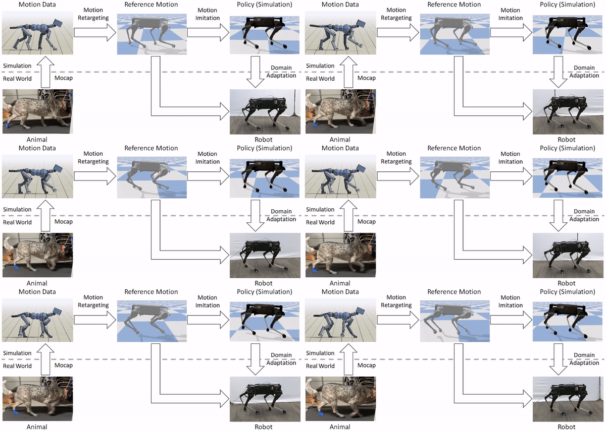
Our framework consists of three main components: motion retargeting, motion imitation, and domain adaptation. 1) First, given a reference motion, the motion retargeting stage maps the motion from the original animal’s morphology to the robot’s morphology. 2) Next, the motion imitation stage uses the retargeted reference motion to train a policy for imitating the motion in simulation. 3) Finally, the domain adaptation stage transfers the policy from simulation to a real robot via a sample efficient domain adaptation process. We apply this framework to learn a variety of agile locomotion skills for a Laikago quadruped robot.


The framework consists of three stages: motion retargeting, motion imitation, and domain adaptation. It receives as input motion data recorded from an animal, and outputs a control policy that enables a robot to reproduce the motion in the real world.

Motion Retargeting

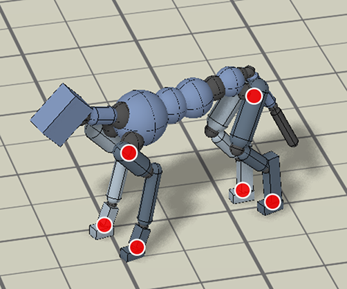
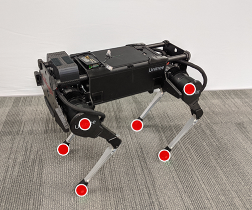
An animal’s body is generally quite different from a robot’s body. So before the robot can imitate the animal’s motion, we must first map the motion to the robot’s body. The goal of the retargeting process is to construct a reference motion for the robot that captures the important characteristics of the animal’s motion. To do this, we first identify a set of source keypoints on the animal’s body, such as the hips and the feet. Then, corresponding target keypoints are specified on the robot’s body.


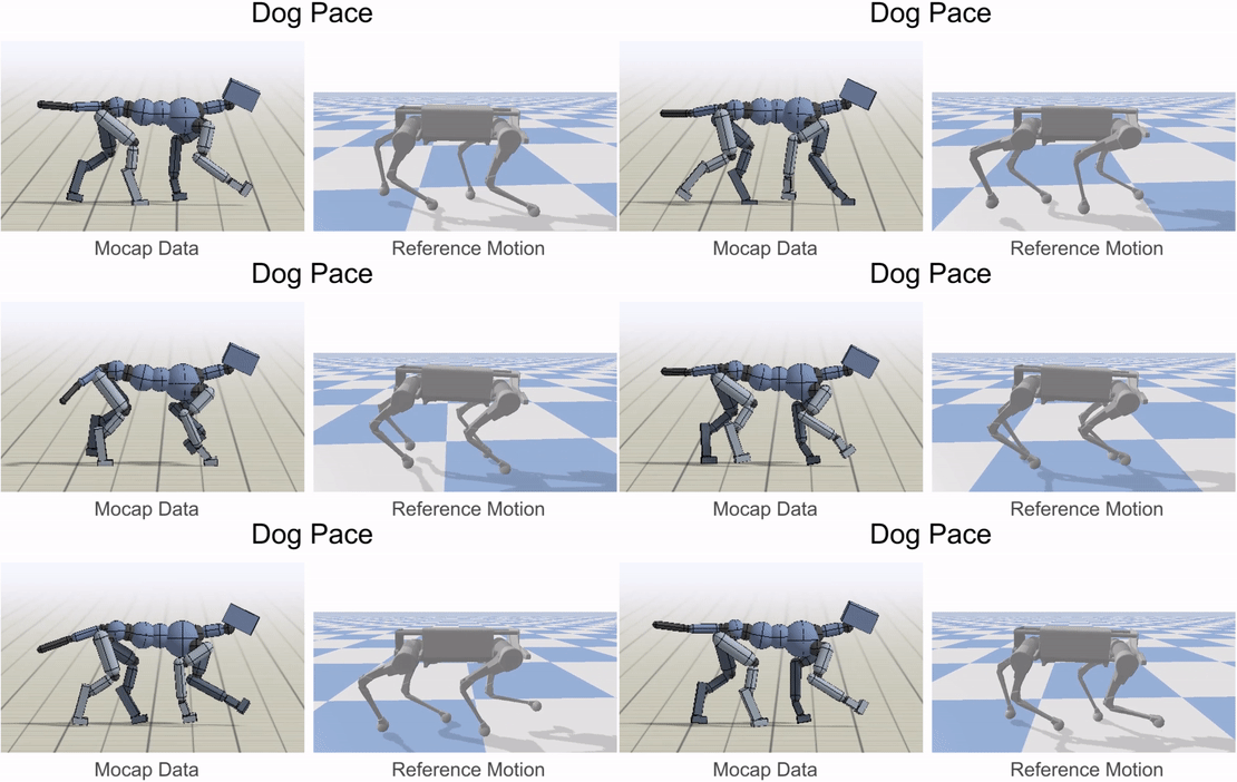
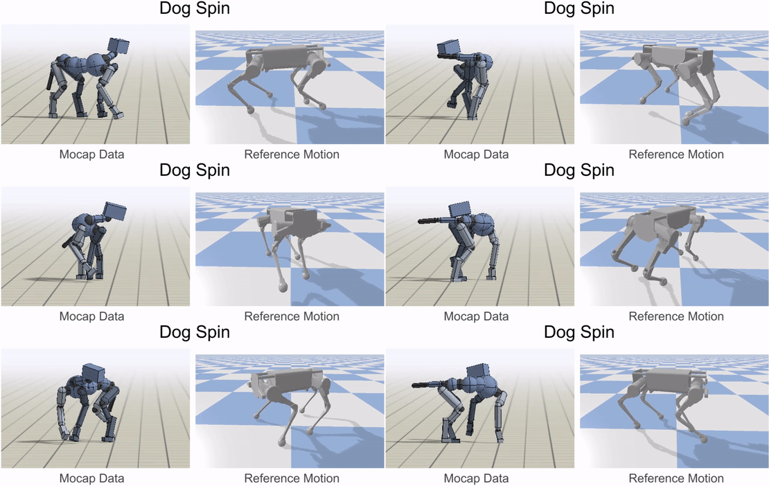
Inverse-kinematics (IK) is used to retarget mocap clips recorded from a real dog (left) to the robot (right). Corresponding pairs of keypoints (red) are specified on the dog and robot’s bodies, and then IK is used to compute a pose for the robot that tracks the keypoints.

Next, inverse-kinematics is used to construct a reference motion for the robot that tracks the corresponding keypoints from the animal at every timestep.


Inverse-kinematics is used to retarget mocap clips recorded from a dog to the robot.

Motion Imitation

After retargeting the reference motion to the robot, the next step is to train a control policy to imitate the retargeted motion. But reinforcement learning algorithms can take a long time to learn an effective policy, and directly training on a real robot can be fairly dangerous (both for the robot and its human companions). So, we instead opt to perform most of the training in the comforts of simulation, and then transfer the learned policy to the real world using more sample efficient adaptation techniques. All simulations are performed using PyBullet.

The policy $\pi(\mathbf{a} | \mathbf{s}, \mathbf{g})$, takes as input a state $\mathbf{s}$, which represents the configuration of the robot’s body, and a goal $\mathbf{g}$, which specifies target poses from the reference motion that the robot is to imitate. It then outputs an action $\mathbf{a}$, which specifies target angles for PD controllers at each of the robot’s joints. To train the policy to imitate a reference motion, we use a reward function that encourages the robot to minimize the difference between the pose of the reference motion $\hat{\mathbf{q}}_t$ and the pose of the simulated character $\mathbf{q}_t$ at every timestep $t$,

By simply using different reference motions in the reward function, we can train a simulated robot to imitate a variety of different skills.


Reinforcement learning is used to train a simulated robot to imitate the retargeted reference motions.

Domain Adaptation

Since simulators generally provide only a coarse approximation of the real world, policies trained in simulation often perform fairly poorly when deployed on a real robot. Therefore, to transfer a policy trained in simulation to the real world, we use a sample efficient domain adaptation techniques that can adapt the policy to the real world using only a small number of trials on the real robot. To do this, we first apply domain randomization during training in simulation, which randomly varies the dynamics parameters, such as mass and friction. The dynamics parameters are then also collected into a vector $\mu$ and encoded into a latent presentation $\mathbf{z}$ by an encoder $E(\mathbf{z} | \mu)$. The latent encoding is passed as an additional input to the policy $\pi(\mathbf{a} | \mathbf{s}, \mathbf{g}, \mathbf{z})$.


The dynamics parameters of the simulation are varied during training, and also encoded into a latent representation that is provided as an additional input to the policy.

When transferring the policy to a real robot, we remove the encoder and directly search for a $\mathbf{z}$ that maximizes the robot’s rewards in the real world. This is done using advantage weighted regression, a simple off-policy reinforcement learning algorithm. In our experiments, this technique is often able to adapt a policy to the real world with less than 50 trials, which corresponds to roughly 8 minutes of real-world data.


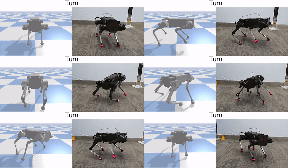
Comparison of policies before and after adaptation on the real robot. Before adaptation, the robot is prone to falling. But after adaptation, the policies are able to more consistently execute the desired skills.

Results

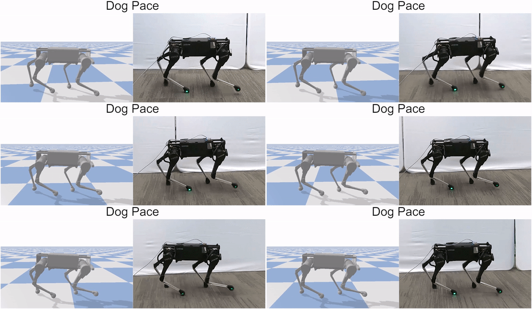
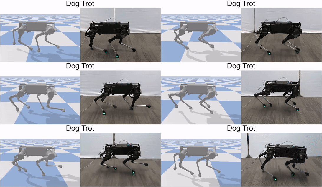
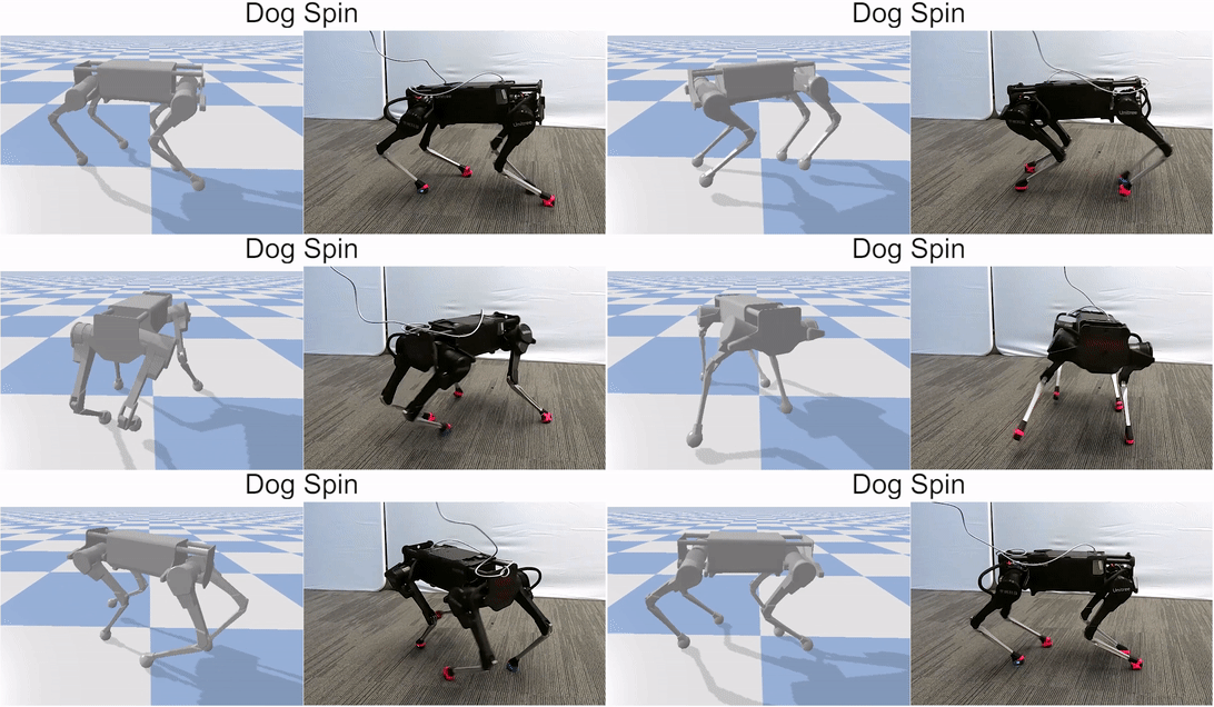
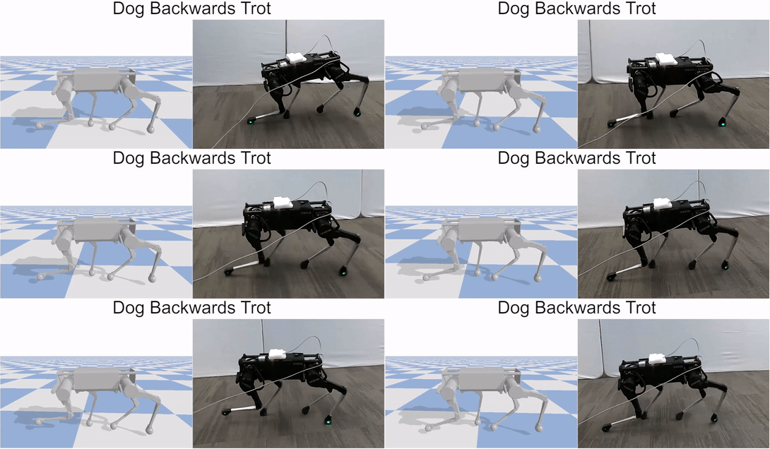
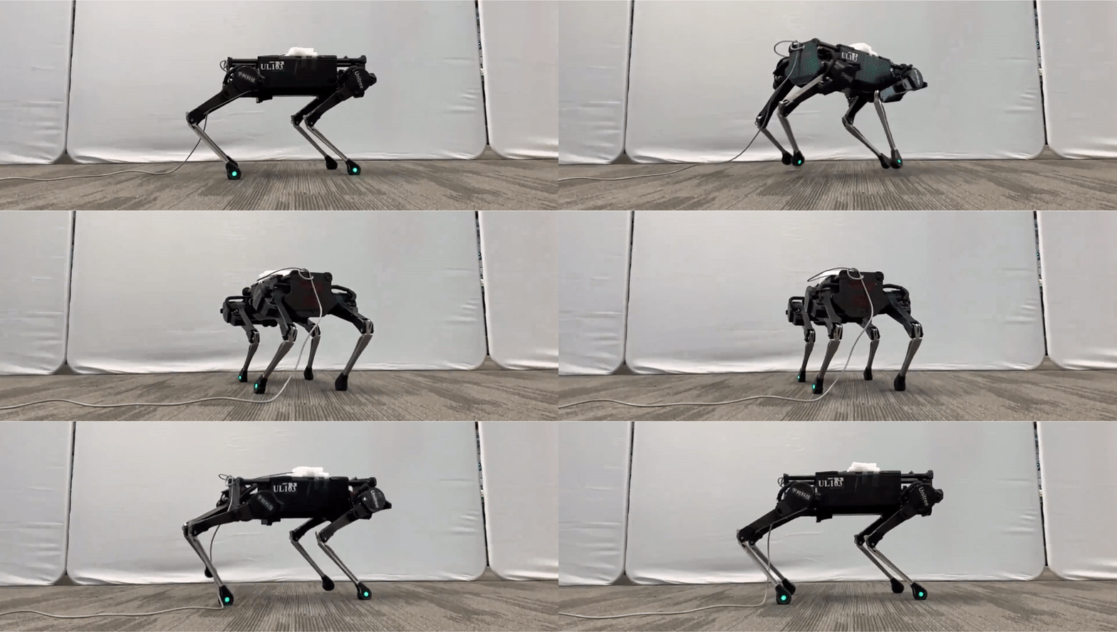
Our framework is able to train a robot to imitate various locomotion skills from a dog, including different walking gaits, such as pacing and trotting, as well as a fast spinning motion. By simply playing the forwards walking motions backwards, we are also able to train the robot to walk backwards.


Laikago imitating various skills from a dog.

In addition to imitating motions from real dogs, we can also imitate artist-animated keyframe motion, including a dynamic hop-turn:


Hop Turn
Skills learned by imitating artist-animated keyframe motions.

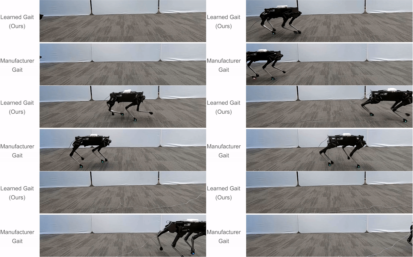
We also compared the learned policies with the manually-designed controllers provided by the manufacturer. Our policies are able to learn faster gaits.

Comparison of learned trotting gait with the built-in gait provided by the manufacturer.

Overall, our system has been able to reproduce a fairly diverse corpus of behaviors with a quadruped robot. However, due to hardware and algorithmic limitations, we have not been able to imitate more dynamic motions such as running and jumping. The learned policies are also not as robust as the best manually-designed controllers. Exploring techniques for further improving the agility and robustness of these learned policies could be a valuable step towards more complex real-world applications. Extending this framework to learn skills from videos would also be an exciting direction, which can substantially increase the volume of data from which robots can learn from.

To learn more, check out the paper and code.

We would like to thank Erwin Coumans, Tingnan Zhang, Tsang-Wei Lee, Jie Tan, Sergey Levine, Byron David, Thinh Nguyen, Gus Kouretas, Krista Reymann, and Bonny Ho for all their support and contribution to this work. This project was done in collaboration with Google Brain. This article was initially published on the BAIR blog, and appears here with the authors’ permission.

Does on-policy data collection fix errors in off-policy reinforcement learning?

Reinforcement learning has seen a great deal of success in solving complex decision making problems ranging from robotics to games to supply chain management to recommender systems. Despite their success, deep reinforcement learning algorithms can be exceptionally difficult to use, due to unstable training, sensitivity to hyperparameters, and generally unpredictable and poorly understood convergence properties. Multiple explanations, and corresponding solutions, have been proposed for improving the stability of such methods, and we have seen good progress over the last few years on these algorithms. In this blog post, we will dive deep into analyzing a central and underexplored reason behind some of the problems with the class of deep RL algorithms based on dynamic programming, which encompass the popular DQN and soft actor-critic (SAC) algorithms – the detrimental connection between data distributions and learned models.

Before diving deep into a description of this problem, let us quickly recap some of the main concepts in dynamic programming. Algorithms that apply dynamic programming in conjunction with function approximation are generally referred to as approximate dynamic programming (ADP) methods. ADP algorithms include some of the most popular, state-of-the-art RL methods such as variants of deep Q-networks (DQN) and soft actor-critic (SAC) algorithms. ADP methods based on Q-learning train action-value functions, $Q(s, a)$, via a Bellman backup. In practice, this corresponds to training a parametric function, $Q_\theta(s, a)$, by minimizing the mean squared difference to a backup estimate of the Q-function, defined as:

$\mathcal{B}^*Q(s, a) = r(s, a) + \gamma \mathbb{E}_{s’|s, a} [\max_{a’} \bar{Q}(s’, a’)],$

where $\bar{Q}$ denotes a previous instance of the original Q-function, $Q_\theta$, and is commonly referred to as a target network. This update is summarized in the equation below.

An analogous update is also used for actor-critic methods that also maintain an explicitly parametrized policy, $\pi_\phi(a|s)$, alongside a Q-function. Such an update typically replaces $\max_{a’}$ with an expectation under the policy, $\mathbb{E}_{a’ \sim \pi_\phi}$. We shall use the $\max_{a’}$ version for consistency throughout, however, the actor-critic version follows analogously. These ADP methods aim at learning the optimal value function, $Q^*$, by applying the Bellman backup iteratively untill convergence.

A central factor that affects the performance of ADP algorithms is the choice of the training data-distribution, $\mathcal{D}$, as shown in the equation above. The choice of $\mathcal{D}$ is an integral component of the backup, and it affects solutions obtained via ADP methods, especially since function approximation is involved. Unlike tabular settings, function approximation causes the learned Q function to depend on the choice of data distribution $\mathcal{D}$, thereby affecting the dynamics of the learning process. We show that on-policy exploration induces distributions $\mathcal{D}$ such that training Q-functions under $\mathcal{D}$ may fail to correct systematic errors in the Q-function, even if Bellman error is minimized as much as possible – a phenomenon that we refer to as an absence of corrective feedback.

Corrective Feedback and Why it is Absent in ADP

What is corrective feedback formally? How do we determine if it is present or absent in ADP methods? In order to build intuition, we first present a simple contextual bandit (one step RL) example, where the Q-function is trained to match $Q^*$ via supervised updates, without bootstrapping. This enjoys corrective feedback, and we then contrast it with ADP methods, which do not. In this example, the goal is to learn the optimal value function $Q^*(s, a)$, which, is equal to the reward $r(s, a)$. At iteration $k$, the algorithm minimizes the estimation error of the Q-function:

$\mathcal{L}(Q) = \mathbb{E}_{s \sim \beta(s), a \sim \pi_k(a|s)}[|Q_k(s, a) – Q^*(s, a)|].$

Using an $\varepsilon$-greedy or Boltzmann policy for exploration, denoted by $\pi_k$, gives rise to a hard negative mining phenomenon – the policy chooses precisely those actions that correspond to possibly over-estimated Q-values for each state $s$ and observes the corresponding, $r(s, a)$ or $Q^*(s, a)$, as a result. Then, minimizing $\mathcal{L}(Q)$, on samples collected this way corrects errors in the Q-function, as $Q_k(s, a)$ is pushed closer to match $Q^*(s, a)$ for actions $a$ with incorrectly high Q-values, correcting precisely the Q-values which may cause sub-optimal performance. This constructive interaction between online data collection and error correction – where the induced online data distribution corrects errors in the value function – is what we refer to as corrective feedback.

In contrast, we will demonstrate that ADP methods that rely on previous Q-functions to generate targets for training the current Q-function, may not benefit from corrective feedback. This difference between bandits and ADP happens because the target values are computed by applying a Bellman backup on the previous Q-function, (target value), rather than the optimal $Q^*$, so, errors in $\bar{Q}$, at the next states can result in incorrect Q-value targets at the current state. No matter how often the current transition is observed, or how accurately Bellman errors are minimized, the error in the Q-value with respect to the optimal Q-function, $|Q – Q^*|$, at this state is not reduced. Furthermore, in order to obtain correct target values, we need to ensure that values at state-action pairs occurring at the tail ends of the data distribution $\mathcal{D}$, which are primary causes of errors in Q-values at other states, are correct. However, as we will show via a simple didactic example, that this correction process may be extremely slow and may not occur, mainly because of undesirable generalization effects of the function approximator.

Let’s consider a didactic example of a tree-structured deterministic MDP with 7 states and 2 actions, $a_1$ and $a_2$, at each state.


Figure 1: Run of an ADP algorithm with on-policy data collection. Boxed nodes and circled nodes denote groups of states aliased by function approximation — values of these nodes are affected due to parameter sharing and function approximation.

A run of an ADP algorithm that chooses the current on-policy state-action marginal as $\mathcal{D}$ on this tree MDP is shown in Figure 1. Thus, the Bellman error at a state is minimized in proportion to the frequency of occurrence of that state in the policy state-action marginal. Since the leaf node states are the least frequent in this on-policy marginal distribution (due to the discounting), the Bellman backup is unable to correct errors in Q-values at such leaf nodes, due to their low frequency and aliasing with other states arising due to function approximation. Using incorrect Q-values at the leaf nodes to generate targets for other nodes in the tree, just gives rise to incorrect values, even if Bellman error is fully minimized at those states. Thus, most of the Bellman updates do not actually bring Q-values at the states of the MDP closer to $Q^*$, since the primary cause of incorrect target values isn’t corrected.

This observation is surprising, since it demonstrates how the choice of an online distribution coupled with function approximation might actually learn incorrect Q-values. On the other hand, a scheme that chooses to update states level by level progressively (Figure 2), ensuring that target values used at any iteration of learning are correct, very easily learns correct Q-values in this example.


Figure 2: Run of an ADP algorithm with an oracle distribution, that updates states level-by level, progressing through the tree from the leaves to the root. Even in the presence of function approximation, selecting the right set of nodes for updates gives rise to correct Q-values.

Consequences of Absent Corrective Feedback

Now, one might ask if an absence of corrective feedback occurs in practice, beyond a simple didactic example and whether it hurts in practical problems. Since visualizing the dynamics of the learning process is hard in practical problems as we did for the didactic example, we instead devise a metric that quantifies our intuition for corrective feedback. This metric, what we call value error, is given by:

Increasing values of imply that the algorithm is pushing Q-values farther away from $Q^*$, which means that corrective feedback is absent, if this happens over a number of iterations. On the other hand, decreasing values of $\mathcal{E}_k$ implies that the algorithm is continuously improving its estimate of $Q$, by moving it towards $Q^*$ with each iteration, indicating the presence of corrective feedback.

Observe in Figure 3, that ADP methods can suffer from prolonged periods where this global measure of error in the Q-function, $\mathcal{E}_k$, is increasing or fluctuating, and the corresponding returns degrade or stagnate, implying an absence of corrective feedback.


Figure 3: Consequences of absent corrective feedback, including (a) sub-optimal convergence, (b) instability in learning and (c) inability to learn with sparse rewards.

In particular, we describe three different consequences of an absence of corrective feedback:

  1. Convergence to suboptimal Q-functions. We find that on-policy sampling can cause ADP to converge to a suboptimal solution, even in the absence of sampling error. Figure 3(a) shows that the value error $\mathcal{E}_k<$ rapidly decreases initially, and eventually converges to a value significantly greater than 0, from which the learning process never recovers.

  2. Instability in the learning process. We observe that ADP with replay buffers can be unstable. For instance, the algorithm is prone to degradation even if the latest policy obtains returns that are very close to the optimal return in Figure 3(b).

  3. Inability to learn with low signal-to-noise ratio. Absence of corrective feedback can also prevent ADP algorithms from learning quickly in scenarios with low signal-to-noise ratio, such as tasks with sparse/noisy rewards as shown in Figure 3(c). Note that this is not an exploration issue, since all transitions in the MDP are provided to the algorithm in this experiment.

Inducing Maximal Corrective Feedback via Distribution Correction

Now that we have defined corrective feedback and gone over some detrimental consequences an absence of it can have on the learning process of an ADP algorithm, what might be some ways to fix this problem? To recap, an absence of corrective feedback occurs when ADP algorithms naively use the on-policy or replay buffer distributions for training Q-functions. One way to prevent this problem is by computing an “optimal” data distribution that provides maximal corrective feedback, and train Q-functions using this distribution? This way we can ensure that the ADP algorithm always enjoys corrective feedback, and hence makes steady learning progress. The strategy we used in our work is to compute this optimal distribution and then perform a weighted Bellman update that re-weights the data distribution in the replay buffer to this optimal distribution (in practice, a tractable approximation is required, as we will see) via importance sampling based techniques.

We will not go into the full details of our derivation in this article, however, we mention the optimization problem used to obtain a form for this optimal distribution and encourage readers interested in the theory to checkout Section 4 in our paper. In this optimization problem, our goal is to minimize a measure of corrective feedback, given by value error $\mathcal{E}_k$, with respect to the distribution $p_k$ used for Bellman error minimization, at every iteration $k$. This gives rise to the following problem:

$\min _{p_{k}} \; \mathbb{E}_{d^{\pi_{k}}}[|Q_{k}-Q^{*}|]$

$\text { s.t. }\;\; Q_{k}=\arg \min _{Q} \mathbb{E}_{p_{k}}\left[\left(Q-\mathcal{B}^{*} Q_{k-1}\right)^{2}\right]$

We show in our paper that the solution of this optimization problem, that we refer to as the optimal distribution, $p_k^*$, is given by:

$p_{k}^*(s, a) \propto \exp \left(-\left|Q_{k}-Q^{*}\right|(s, a)\right) \frac{\left|Q_{k}-\mathcal{B}^{*} Q_{k-1}\right|(s, a)}{\lambda^{*}}$

By simplifying this expression, we obtain a practically viable expression for weights, $w_k$, at any iteration $k$ that can be used to re-weight the data distribution:

$w_{k}(s, a) \propto \exp \left(-\frac{\gamma \mathbb{E}_{s’|s, a} \mathbb{E}_{a’ \sim \pi_\phi(\cdot|s’)} \Delta_{k-1}(s’, a’)}{\tau}\right)$

where $\Delta_k$ is the accumulated Bellman error over iterations, and it satisfies a convenient recursion making it amenable to practical implementations,

$\Delta_{k}(s, a) =\left|Q_{k}-\mathcal{B}^{*} Q_{k-1}\right|(s, a) +\gamma \mathbb{E}_{s’|s, a} \mathbb{E}_{a’ \sim \pi_\phi(\cdot|s’)} \Delta_{k-1}(s’, a’)$

and $\pi_\phi$ is the Boltzmann or $\varepsilon-$greedy policy corresponding to the current Q function.

What does this expression for $w_k$ intuitively correspond to? Observe that the term appearing in the exponent in the expression for $w_k$ corresponds to the accumulated Bellman error in the target values. Our choice of $w_k$, thus, basically down-weights transitions with highly incorrect target values. This technique falls into a broader class of abstention based techniques that are common in supervised learning settings with noisy labels, where down-weighting datapoints (transitions here) with errorful labels (target values here) can boost generalization and correctness properties of the learned model.


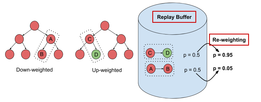
Figure 4: Schematic of the DisCor algorithm. Transitions with errorful target values are downweighted.

Why does our choice of $\Delta_k$, i.e. the sum of accumulated Bellman errors suffice? This is because this value $\Delta_k$ accounts for how error is propagated in ADP methods. Bellman errors, $|Q_k – \mathcal{B}^*Q_{k-1}|$ are propagated under the current policy $\pi_{k-1}$, and then discounted when computing target values for updates in ADP. $\Delta_k$ captures exactly this, and therefore, using this estimate in our weights suffices.

Our practical algorithm, that we refer to as DisCor (Distribution Correction), is identical to conventional ADP methods like Q-learning, with the exception that it performs a weighted Bellman backup – it assigns a weight $w_k(s,a)$ to a transition, $(s, a, r, s’)$ and performs a Bellman backup weighted by these weights, as shown below.

We depict the general principle in the schematic diagram shown in Figure 4.

How does DisCor perform in practice?

We finally present some results that demonstrate the efficacy of our method, DisCor, in practical scenarios. Since DisCor only modifies the chosen distribution for the Bellman update, it can be applied on top of any standard ADP algorithm including soft actor-critic (SAC) or deep Q-network (DQN). Our paper presents results for a number of tasks spanning a wide variety of settings including robotic manipulation tasks, multi-task reinforcement learning tasks, learning with stochastic and noisy rewards, and Atari games. In this blog post, we present two of these results from robotic manipulation and multi-task RL.

  1. Robotic manipulation tasks. On six challenging benchmark tasks from the MetaWorld suite, we observe that DisCor when combined with SAC greatly outperforms prior state-of-the-art RL algorithms such as soft actor-critic (SAC) and prioritized experience replay (PER) which is a prior method that prioritizes states with high Bellman error during training. Note that DisCor usually starts learning earlier than other methods compared to. DisCor outperforms vanilla SAC by a factor of about 50% on average, in terms of success rate on these tasks.


  2. Multi-task reinforcement learning. We also present certain results on the Multi-task 10 (MT10) and Multi-task 50 (MT50) benchmarks from the Meta-world suite. The goal here is to learn a single policy that can solve a number of (10 or 50, respectively) different manipulation tasks that share common structure. We note that DisCor outperforms, state-of-the-art SAC algorithm on both of these benchmarks by a wide margin (for e.g. 50% on MT10, success rate). Unlike the learning process of SAC that tends to plateau over the course of learning, we observe that DisCor always exhibits a non-zero gradient for the learning process, until it converges.


In our paper, we also perform evaluations on other domains such as Atari games and OpenAI gym benchmarks, and we encourage the readers to check those out. We also perform an analysis of the method on tabular domains, understanding different aspects of the method.

Perspectives, Future Work and Open Problems

Some of our and other prior work has highlighted the impact of the data distribution on the performance of ADP algorithms, We observed in another prior work that in contrast to the intuitive belief about the efficacy of online Q-learning with on-policy data collection, Q-learning with a uniform distribution over states and actions seemed to perform best. Obtaining a uniform distribution over state-action tuples during training is not possible in RL, unless all states and actions are observed at least once, which may not be the case in a number of scenarios. We might also ask the question about whether the uniform distribution is the best choice that can be used in an RL setting? The form of the optimal distribution derived in Section 4 of our paper, is a potentially better choice since it is customized to the MDP under consideration.

Furthermore, in the domain of purely offline reinforcement learning, studied in our prior work and some other works, such as this and this, we observe that the data distribution is again a central feature, where backing up out-of-distribution actions and the inability to try these actions out in the environment to obtain answers to counterfactual queries, can cause error accumulation and backups to diverge. However, in this work, we demonstrate a somewhat counterintuitive finding: even with on-policy data collection, where the algorithm, in principle, can evaluate all forms of counterfactual queries, the algorithm may not obtain a steady learning progress, due to an undesirable interaction between the data distribution and generalization effects of the function approximator.


What might be a few promising directions to pursue in future work?

Formal analysis of learning dynamics: While our study is an initial foray into the role that data distributions play in the learning dynamics of ADP algorithms, this motivates a significantly deeper direction of future study. We need to answer questions related to how deep neural network based function approximators actually behave, which are behind these ADP methods, in order to get them to enjoy corrective feedback.

Re-weighting to supplement exploration in RL problems: Our work depicts the promise of re-weighting techniques as a practically simple replacement for altering entire exploration strategies. We believe that re-weighting techniques are very promising as a general tool in our toolkit to develop RL algorithms. In an online RL setting, re-weighting can help remove the some of the burden off exploration algorithms, and can thus, potentially help us employ complex exploration strategies in RL algorithms.

More generally, we would like to make a case of analyzing effects of data distribution more deeply in the context of deep RL algorithms. It is well known that narrow distributions can lead to brittle solutions in supervised learning that also do not generalize. What is the corresponding analogue in reinforcement learning? Distributional robustness style techniques have been used in supervised learning to guarantee a uniformly convergent learning process, but it still remains unclear how to apply these in an RL with function approximation setting. Part of the reason is that the theory of RL often derives from tabular settings, where distributions do not hamper the learning process to the extent they do with function approximation. However, as we showed in this work, choosing the right distribution may lead to significant gains in deep RL methods, and therefore, we believe, that this issue should be studied in more detail.


This blog post is based on our recent paper:

  • DisCor: Corrective Feedback in Reinforcement Learning via Distribution Correction
    Aviral Kumar, Abhishek Gupta, Sergey Levine
    arXiv

We thank Sergey Levine and Marvin Zhang for their valuable feedback on this blog post.


This article was initially published on the BAIR blog, and appears here with the authors’ permission.
Emergent behavior by minimizing chaos

By Glen Berseth

All living organisms carve out environmental niches within which they can maintain relative predictability amidst the ever-increasing entropy around them (1), (2). Humans, for example, go to great lengths to shield themselves from surprise — we band together in millions to build cities with homes, supplying water, food, gas, and electricity to control the deterioration of our bodies and living spaces amidst heat and cold, wind and storm. The need to discover and maintain such surprise-free equilibria has driven great resourcefulness and skill in organisms across very diverse natural habitats. Motivated by this, we ask: could the motive of preserving order amidst chaos guide the automatic acquisition of useful behaviors in artificial agents?

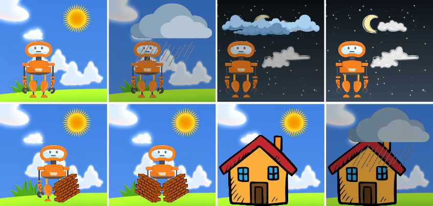
How might an agent in an environment acquire complex behaviors and skills with no external supervision? This central problem in artificial intelligence has evoked several candidate solutions, largely focusing on novelty-seeking behaviors (3), (4), (5). In simulated worlds, such as video games, novelty-seeking intrinsic motivation can lead to interesting and meaningful behavior. However, these environments may be fundamentally lacking compared to the real world. In the real world, natural forces and other agents offer bountiful novelty. Instead, the challenge in natural environments is allostasis: discovering behaviors that enable agents to maintain an equilibrium (homeostasis), for example to preserve their bodies, their homes, and avoid predators and hunger. In the example below we shown an example where an agent is experiencing random events due to the changing weather. If the agent learns to build a shelter, in this case a house, the agent will reduce the observed effects from weather.

We formalize homeostasis as an objective for reinforcement learning based on surprise minimization (SMiRL). In entropic and dynamic environments with undesirable forms of novelty, minimizing surprise (i.e., minimizing novelty) causes agents to naturally seek an equilibrium that can be stably maintained.

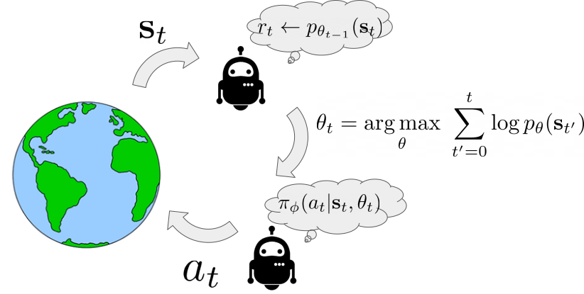
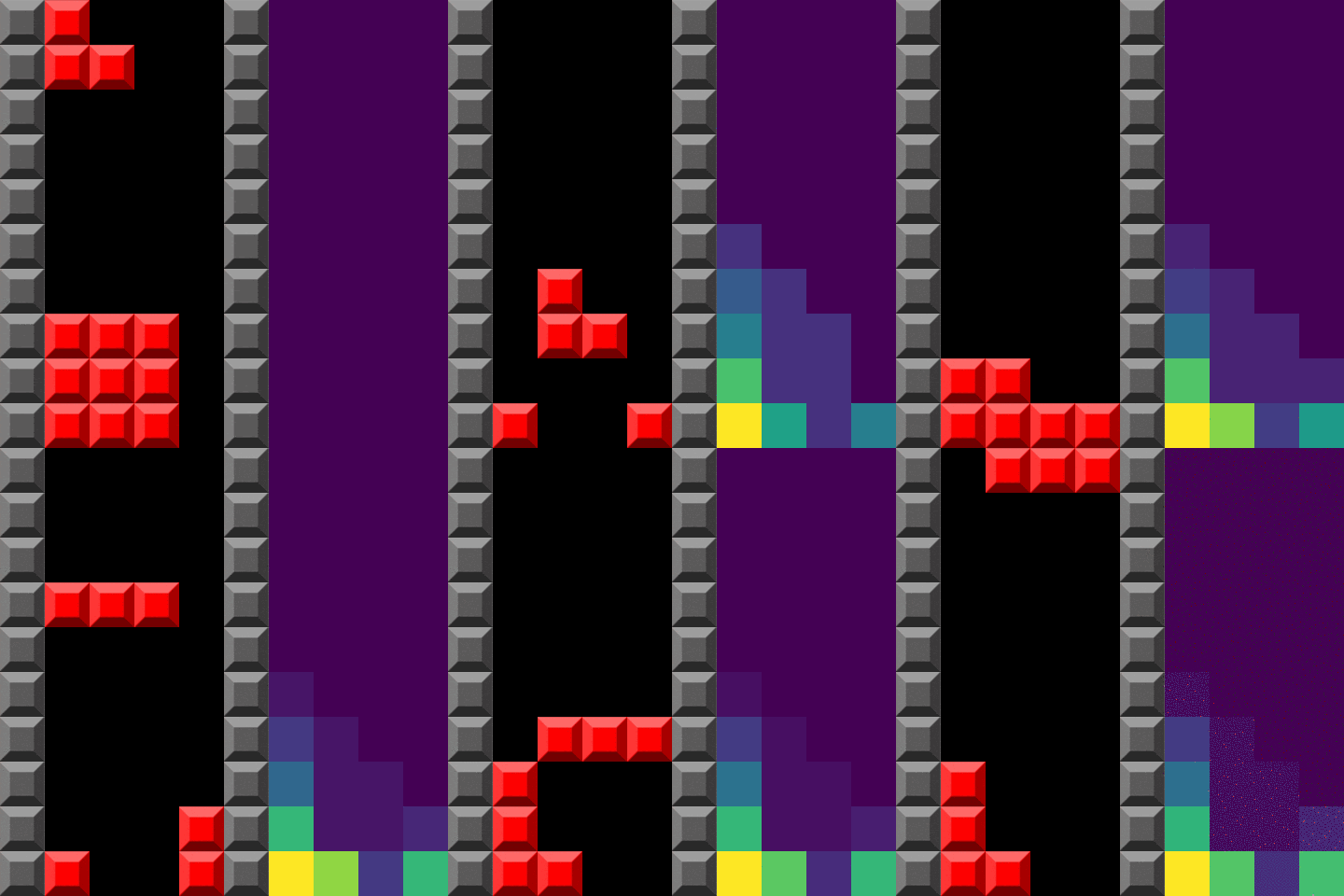
Here we show an illustration of the agent interaction loop using SMiRL. When the agent observes a state $\mathbf{s}$, it computes the probability of this new state given the belief the agent has $r_{t} \leftarrow p_{\theta_{t-1}}(\textbf{s})$. This belief models the states the agent is most familiar with – i.e., the distribution of states it has seen in the past. Experiencing states that are more familiar will result in higher reward. After the agent experience a new state it updates its belief $p_{\theta_{t-1}}(\textbf{s})$ over states to include the most recent experience. Then, the goal of the action policy $\pi(a|\textbf{s}, \theta_{t})$ is to choose actions that will result in the agent consistently experiencing familiar states. Crucially, the agent understands that its beliefs will change in the future. This means that it has two mechanisms by which to maximize this reward: taking actions to visit familiar states, and taking actions to visit states that will change its beliefs such that future states are more familiar. It is this latter mechanism that results in complex emergent behavior. Below, we visualize a policy trained to play the game of Tetris. On the left the blocks the agent chooses are shown and on the right is a visualization of $p_{\theta_{t}}(\textbf{s})$. We can see how as the episode progresses the belief over possible locations to place blocks tends to favor only the bottom row. This encourages the agent to eliminate blocks to prevent board from filling up.


Left: Tetris. Right: HauntedHouse.

Emergent behavior

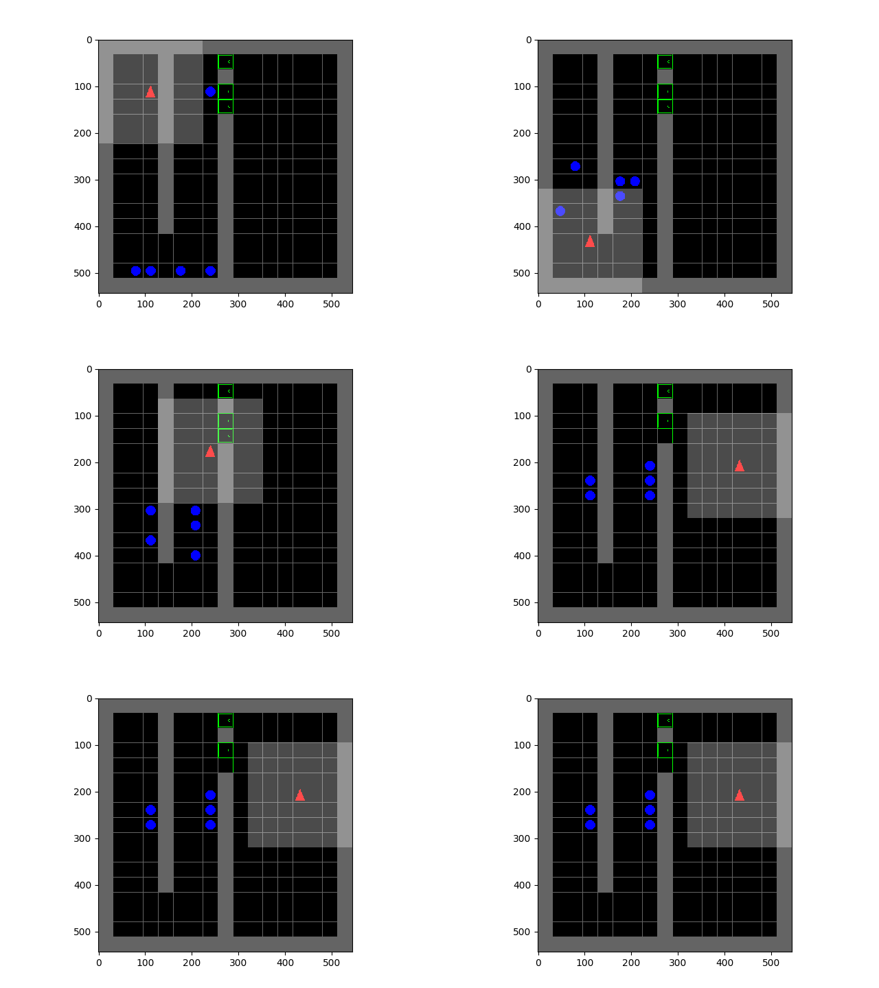
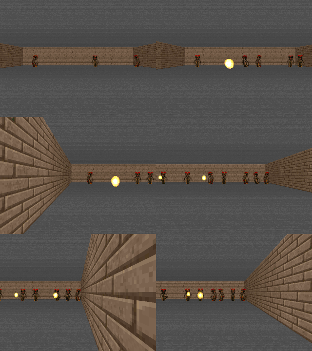
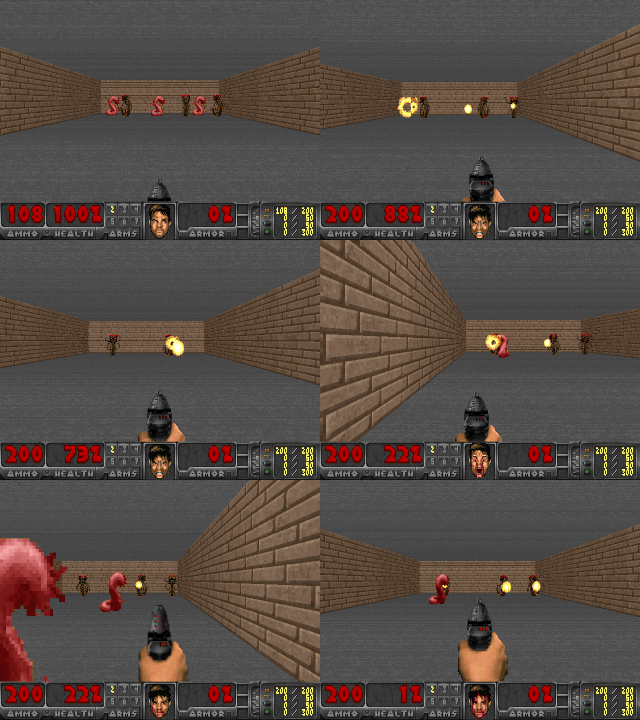
The SMiRL agent demonstrates meaningful emergent behaviors in a number of different environments. In the Tetris environment, the agent is able to learn proactive behaviors to eliminate rows and properly play the game. The agent also learns emergent game playing behavior in the VizDoom environment, acquiring an effective policy for dodging the fireballs thrown by the enemies. In both of these environments, stochastic and chaotic events force the SMiRL agent to take a coordinated course of action to avoid unusual states, such as full Tetris boards or fireball explorations.


Left: Doom Hold The Line. Right: Doom Defend The Line.

Biped

In the Cliff environment, the agent learns a policy that greatly reduces the probability of falling off of the cliff by bracing against the ground and stabilize itself at the edge, as shown in the figure below. In the Treadmill environment, SMiRL learns a more complex locomotion behavior, jumping forward to increase the time it stays on the treadmill, as shown in figure below.


Left: Cliff. Right: Treadmill.

Comparison to Intrinsic motivation:

Intrinsic motivation is the idea that behavior is driven by internal reward signals that are task independent. Below, we show plots of the environment-specific rewards over time on Tetris, VizDoomTakeCover, and the humanoid domains. In order to compare SMiRL to more standard intrinsic motivation methods, which seek out states that maximize surprise or novelty, we also evaluated ICM (5) and RND (6). We include an oracle agent that directly optimizes the task reward. On Tetris, after training for $2000$ epochs, SMiRL achieves near perfect play, on par with the oracle reward optimizing agent, with no deaths. ICM seeks novelty by creating more and more distinct patterns of blocks rather than clearing them, leading to deteriorating game scores over time. On VizDoomTakeCover, SmiRL effectively learns to dodge fireballs thrown by the adversaries.

The baseline comparisons for the Cliff and Treadmill environments have a similar outcome. The novelty seeking behavior of ICM causes it to learn a type of irregular behavior that causes the agent to jump off the Cliff and roll around on the Treadmill, maximizing the variety (and quantity) of falls.

SMiRL + Curiosity:

While on the surface, SMiRL minimizes surprise and curiosity approaches like ICM maximize novelty, they are in fact not mutually incompatible. In particular, while ICM maximizes novelty with respect to a learned transition model, SMiRL minimizes surprise with respect to a learned state distribution. We can combine ICM and SMiRL to achieve even better results on the Treadmill environment.


Left: Treadmill+ICM. Right: Pedestal.

Insights:

The key insight utilized by our method is that, in contrast to simple simulated domains, realistic environments exhibit dynamic phenomena that gradually increase entropy over time. An agent that resists this growth in entropy must take active and coordinated actions, thus learning increasingly complex behaviors. This is different from commonly proposed intrinsic exploration methods based on novelty, which instead seek to visit novel states and increase entropy. SMiRL holds promise for a new kind of unsupervised RL method that produces behaviors that are closely tied to the prevailing disruptive forces, adversaries, and other sources of entropy in the environment.

This article was initially published on the BAIR blog, and appears here with the author’s permission.

Data-driven deep reinforcement learning

By Aviral Kumar

One of the primary factors behind the success of machine learning approaches in open world settings, such as image recognition and natural language processing, has been the ability of high-capacity deep neural network function approximators to learn generalizable models from large amounts of data. Deep reinforcement learning methods, however, require active online data collection, where the model actively interacts with its environment. This makes such methods hard to scale to complex real-world problems, where active data collection means that large datasets of experience must be collected for every experiment – this can be expensive and, for systems such as autonomous vehicles or robots, potentially unsafe. In a number of domains of practical interest, such as autonomous driving, robotics, and games, there exist plentiful amounts of previously collected interaction data which, consists of informative behaviours that are a rich source of prior information. Deep RL algorithms that can utilize such prior datasets will not only scale to real-world problems, but will also lead to solutions that generalize substantially better. A data-driven paradigm for reinforcement learning will enable us to pre-train and deploy agents capable of sample-efficient learning in the real-world.

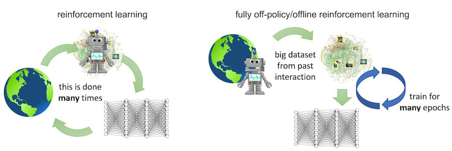
In this work, we ask the following question: Can deep RL algorithms effectively leverage prior collected offline data and learn without interaction with the environment? We refer to this problem statement as fully off-policy RL, previously also called batch RL in literature. A class of deep RL algorithms, known as off-policy RL algorithms can, in principle, learn from previously collected data. Recent off-policy RL algorithms such as Soft Actor-Critic (SAC), QT-Opt, and Rainbow, have demonstrated sample-efficient performance in a number of challenging domains such as robotic manipulation and atari games. However, all of these methods still require online data collection, and their ability to learn from fully off-policy data is limited in practice. In this work, we show why existing deep RL algorithms can fail in the fully off-policy setting. We then propose effective solutions to mitigate these issues.

Read More

RoboNet: A dataset for large-scale multi-robot learning

By Sudeep Dasari

This post is cross-listed at the SAIL Blog and the CMU ML blog.

In the last decade, we’ve seen learning-based systems provide transformative solutions for a wide range of perception and reasoning problems, from recognizing objects in images to recognizing and translating human speech. Recent progress in deep reinforcement learning (i.e. integrating deep neural networks into reinforcement learning systems) suggests that the same kind of success could be realized in automated decision making domains. If fruitful, this line of work could allow learning-based systems to tackle active control tasks, such as robotics and autonomous driving, alongside the passive perception tasks to which they have already been successfully applied.

While deep reinforcement learning methods – like Soft Actor Critic – can learn impressive motor skills, they are challenging to train on large and broad data that is not from the target environment. In contrast, the success of deep networks in fields like computer vision was arguably predicated just as much on large datasets, such as ImageNet, as it was on large neural network architectures. This suggests that applying data-driven methods to robotics will require not just the development of strong reinforcement learning methods, but also access to large and diverse datasets for robotics. Not only can large datasets enable models that generalize effectively, but they can also be used to pre-train models that can then be adapted to more specialized tasks using much more modest datasets. Indeed, “ImageNet pre-training” has become a default approach for tackling diverse tasks with small or medium datasets – like 3D building reconstruction. Can the same kind of approach be adopted to enable broad generalization and transfer in active control domains, such as robotics?

Unfortunately, the design and adoption of large datasets in reinforcement learning and robotics has proven challenging. Since every robotics lab has their own hardware and experimental set-up, it is not apparent how to move towards an “ImageNet-scale” dataset for robotics that is useful for the entire research community. Hence, we propose to collect data across multiple different settings, including from varying camera viewpoints, varying environments, and even varying robot platforms. Motivated by the success of large-scale data-driven learning, we created RoboNet, an extensible and diverse dataset of robot interaction collected across four different research labs. The collaborative nature of this work allows us to easily capture diverse data in various lab settings across a wide variety of objects, robotic hardware, and camera viewpoints. Finally, we find that pre-training on RoboNet offers substantial performance gains compared to training from scratch in entirely new environments.


Our goal is to pre-train reinforcement learning models on a sufficiently diverse dataset and then transfer knowledge (either zero-shot or with fine-tuning) to a different test environment.

Collecting RoboNet

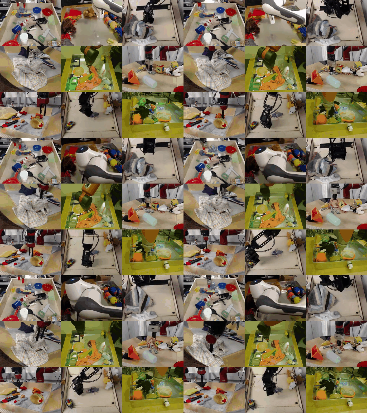
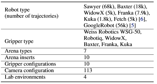
RoboNet consists of 15 million video frames, collected by different robots interacting with different objects in a table-top setting. Every frame includes the image recorded by the robot’s camera, arm pose, force sensor readings, and gripper state. The collection environment, including the camera view, the appearance of the table or bin, and the objects in front of the robot are varied between trials. Since collection is entirely autonomous, large amounts can be cheaply collected across multiple institutions. A sample of RoboNet along with data statistics is shown below:


A sample of data from RoboNet alongside a summary of the current dataset. Note that any GIF compression artifacts in this animation are not present in the dataset itself.

How can we use RoboNet?

After collecting a diverse dataset, we experimentally investigate how it can be used to enable general skill learning that transfers to new environments. First, we pre-train visual dynamics models on a subset of data from RoboNet, and then fine-tune them to work in an unseen test environment using a small amount of new data. The constructed test environments (one of which is visualized below) all include different lab settings, new cameras and viewpoints, held-out robots, and novel objects purchased after data collection concluded.


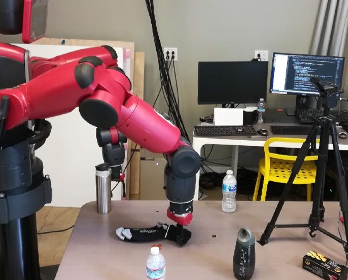
Example test environment constructed in a new lab, with a temporary uncalibrated camera, and a new Baxter robot. Note that while Baxters are present in RoboNet that data is not included during model pre-training.

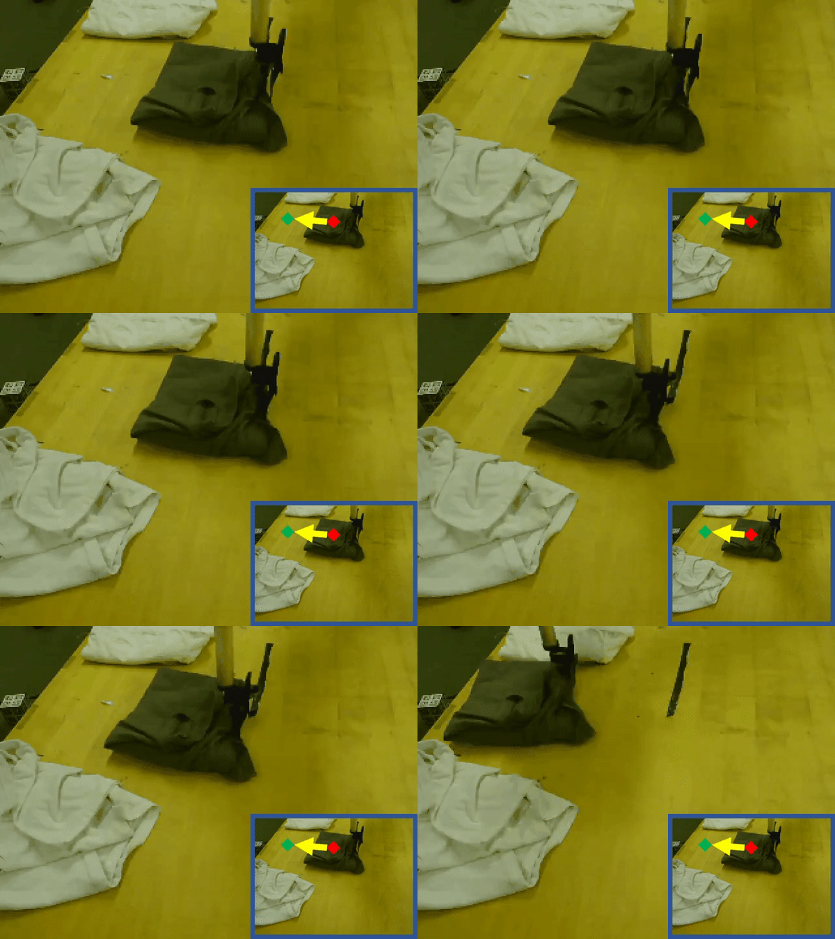
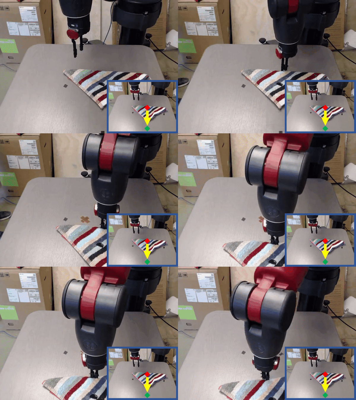
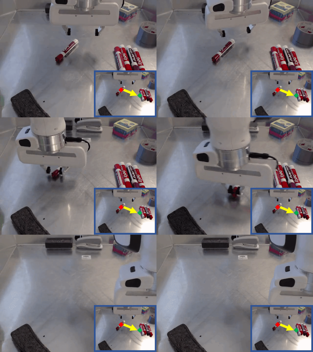
After tuning, we deploy the learned dynamics models in the test environment to perform control tasks – like picking and placing objects – using the visual foresight model based reinforcement learning algorithm. Below are example control tasks executed in various test environments.


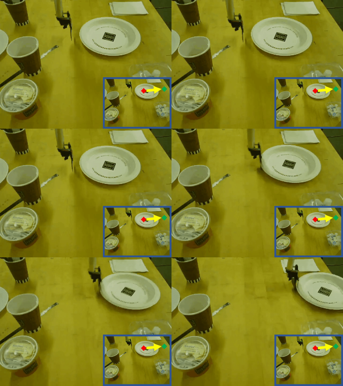
Kuka can align shirts next to the others

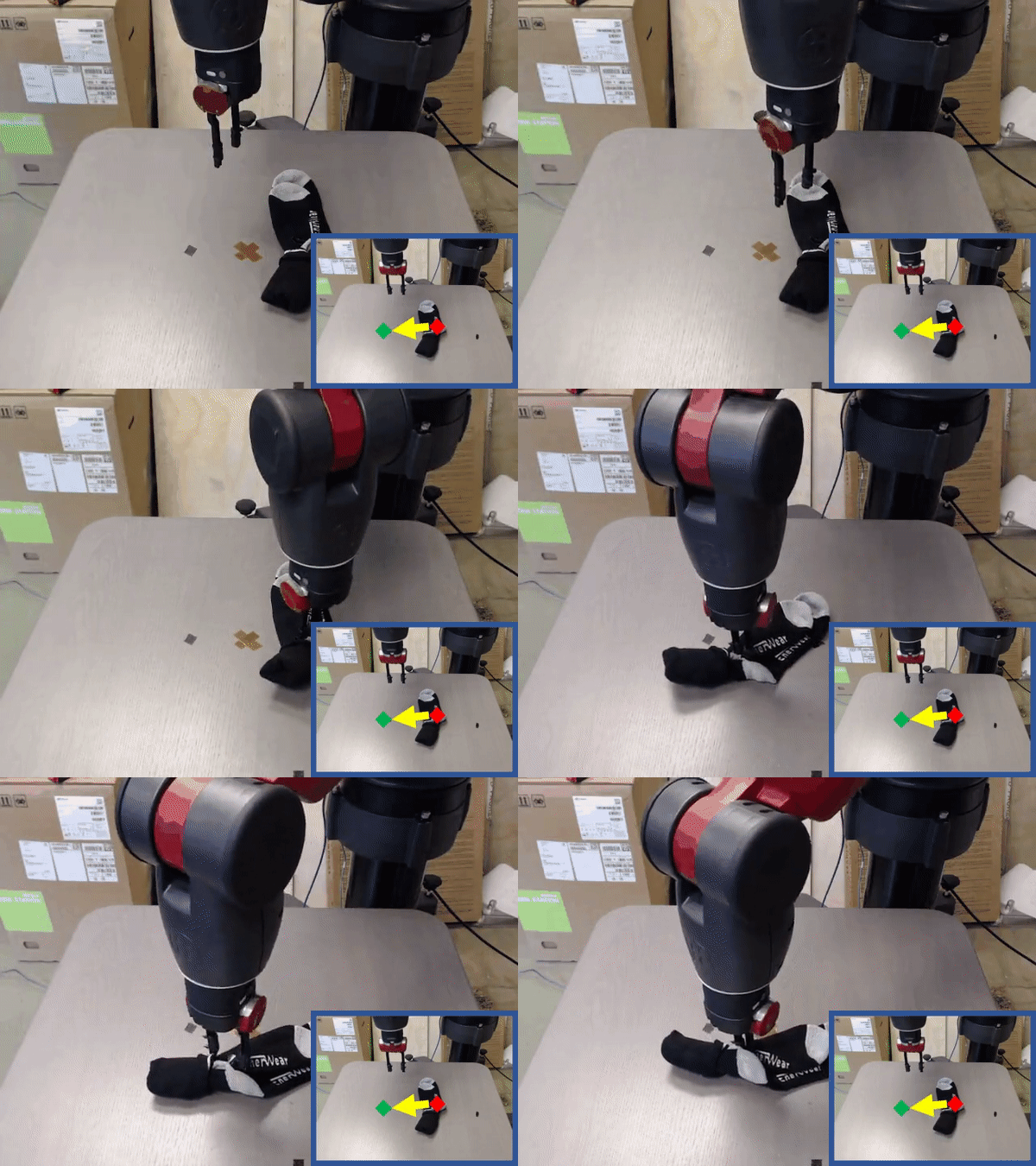
Baxter can sweep the table with cloth

Franka can grasp and reposition the markers


Kuka can move the plate to the edge of the table

Baxter can pick up and reposition socks

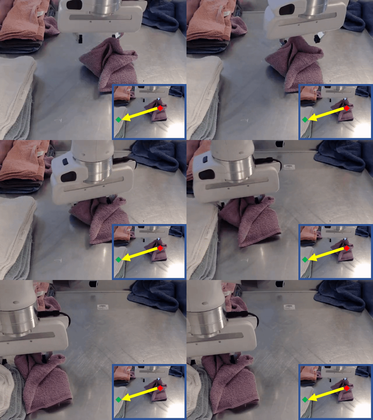
Franka can stack the towel on the pile


Here you can see examples of visual foresight fine-tuned to perform basic control tasks in three entirely different environments. For the experiments, the target robot and environment was subtracted from RoboNet during pre-training. Fine-tuning was accomplished with data collected in one afternoon.

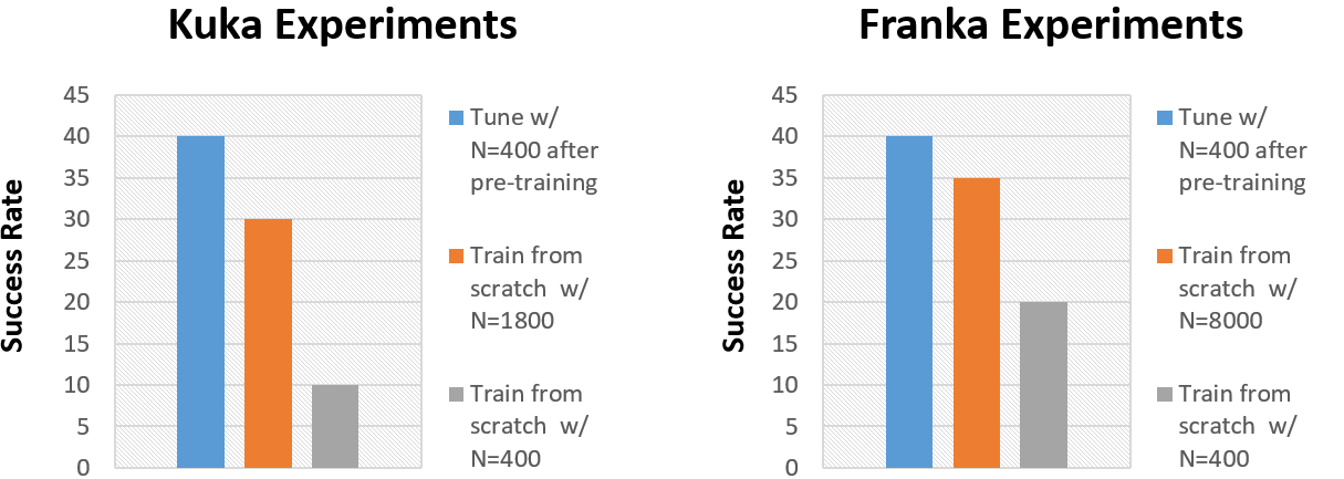
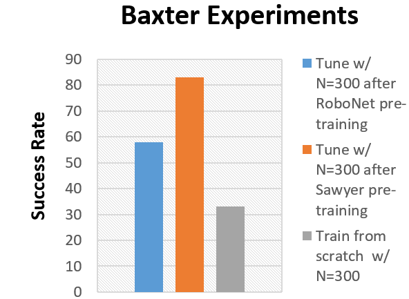
We can now numerically evaluate if our pre-train controllers can pick up skills in new environments faster than a randomly initialized one. In each environment, we use a standard set of benchmark tasks to compare the performance of our pre-trained controller against the performance of a model trained only on data from the new environment. The results show that the fine-tuned model is ~4x more likely to complete the benchmark task than the one trained without RoboNet. Impressively, the pre-trained models can even slightly outperform models trained from scratch on significantly (5-20x) more data from the test environment. This suggests that transfer from RoboNet does indeed offer large performance gains compared to training from scratch!


We compare the performance of fine-tuned models against their counterparts trained from scratch in two different test environments (with different robot platforms).

Clearly fine-tuning is better than training from scratch, but is training on all of RoboNet always the best way to go? To test this, we compare pre-training on various subsets of RoboNet versus training from scratch. As seen before, the model pre-trained on all of RoboNet (excluding the Baxter platform) performs substantially better than the random initialization model. However, the “RoboNet pre-trained” model is outperformed by a model trained on a subset of RoboNet data collected on the Sawyer robot – the single-arm variant of Baxter.


Models pre-trained on various subsets of RoboNet are compared to one trained from scratch in an unseen (during pre-training) Baxter control environment

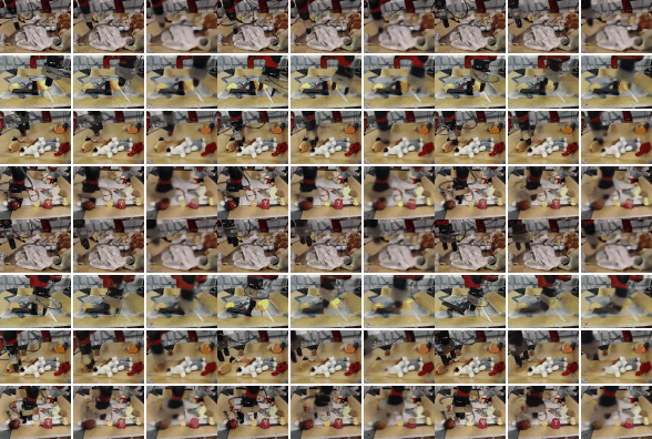
The similarities between the Baxter and Sawyer likely partly explain our results, but why does simply adding data to the training set hurt performance after fine-tuning? We theorize that this effect occurs due to model under-fitting. In other words, RoboNet is an extremely challenging dataset for a visual dynamics model, and imperfections in the model predictions result in bad control performance. However, larger models with more parameters tend to be more powerful, and thus make better predictions on RoboNet (visualized below). Note that increasing the number of parameters greatly improves prediction quality, but even large models with 500M parameters (middle column in the videos below) are still quite blurry. This suggests ample room for improvement, and we hope that the development of newer more powerful models will translate to better control performance in the future.


We compare video prediction models of various size trained on RoboNet. A 75M parameter model (right-most column) generates significantly blurrier predictions than a large model with 500M parameters (center column).

Final Thoughts

This work takes the first step towards creating learned robotic agents that can operate in a wide range of environments and across different hardware. While our experiments primarily explore model-based reinforcement learning, we hope that RoboNet will inspire the broader robotics and reinforcement learning communities to investigate how to scale model-based or model-free RL algorithms to meet the complexity and diversity of the real world.

Since the dataset is extensible, we encourage other researchers to contribute the data generated from their experiments back into RoboNet. After all, any data containing robot telemetry and video could be useful to someone else, so long as it contains the right documentation. In the long term, we believe this process will iteratively strengthen the dataset, and thus allow our algorithms that use it to achieve greater levels of generalization across tasks, environments, robots, and experimental set-ups.

For more information please refer to the the project website. We’ve also open sourced our code-base and the entire RoboNet dataset.

Finally, I would like to thank Sergey Levine, Chelsea Finn, and Frederik Ebert for their helpful feedback on this post.

This article was initially published on the BAIR blog, and appears here with the authors’ permission.
This blog post was based on the following paper:

Look then listen: Pre-learning environment representations for data-efficient neural instruction following

By David Gaddy

When learning to follow natural language instructions, neural networks tend to be very data hungry – they require a huge number of examples pairing language with actions in order to learn effectively. This post is about reducing those heavy data requirements by first watching actions in the environment before moving on to learning from language data. Inspired by the idea that it is easier to map language to meanings that have already been formed, we introduce a semi-supervised approach that aims to separate the formation of abstractions from the learning of language.

Empirically, we find that pre-learning of patterns in the environment can help us learn grounded language with much less data.

Before we dive into the details, let’s look at an example to see why neural networks struggle to learn from smaller amounts of data. For now, we’ll use examples from the SHRDLURN block stacking task, but later we’ll look at results on another environment.

Let’s put ourselves in the shoes of a model that is learning to follow instructions. Suppose we are given the single training example below, which pairs a language command with an action in the environment:

This example tells us that if we are in state (a) and are trying to follow the instruction (b), the correct output for our model is the state (c). Before learning, the model doesn’t know anything about language, so we must rely on examples like the one shown to figure out the meaning of the words. After learning, we will be given new environment states and new instructions, and the model’s job is to choose the correct output states from executing the instructions. First let’s consider a simple case where we get the exact same language, but the environment state is different, like the one shown here:

On this new state, the model has many different possible outputs that it could consider. Here are just a few:

Some of these outputs seem reasonable to a human, like stacking red blocks on orange blocks or stacking red blocks on the left, but others are kind of strange, like generating a completely unrelated configuration of blocks. To a neural network with no prior knowledge, however, all of these options look plausible.

A human learning a new language might approach this task by reasoning about possible meanings of the language that are consistent with the given example and choosing states that correspond to those meanings. The set of possible meanings to consider comes from prior knowledge about what types of things might happen in an environment and how we can talk about them. In this context, a meaning is an abstract transformation that we can apply to states to get new states. For example, if someone saw the training instance above paired with language they didn’t understand, they might focus on two possible meanings for the instruction: it could be telling us to stack red blocks on orange blocks, or it could be telling us to stack a red block on the leftmost position.

Although we don’t know which of these two options is correct – both are plausible given the evidence – we now have many fewer options and might easily distinguish between them with just one or two more related examples. Having a set of pre-formed meanings makes learning easier because the meanings constrain the space of possible outputs that must be considered.

In fact, pre-formed meanings do even more than just restricting the number of choices, because once we have chosen a meaning to pair with the language, it specifies the correct way to generalize across a wide variety of different initial environment states. For example, consider the following transitions:

If we know in advance that all of these transitions belong together in a single semantic group (adding a red block on the left), learning language becomes easier because we can map to the group instead of the individual transitions. An end-to-end network that doesn’t start with any grouping of transitions has a much harder time because it has to learn the correct way to generalize across initial states. One approach used by a long line of past work has been to provide the learner with a manually defined set of abstractions called logical forms. In contrast, we take a more data-driven approach where we learn abstractions from unsupervised (language-free) data instead.

In this work, we help a neural network learn language with fewer examples by first learning abstractions from language-free observations of actions in an environment. The idea here is that if the model sees lots of actions happening in an environment, perhaps it can pick up on patterns in what tends to be done, and these patterns might give hints at what abstractions are useful. Our pre-learned abstractions can make language learning easier by constraining the space of outputs we need to consider and guiding generalization across different environment states.

We break up learning into two phases: an environment learning phase where our agent builds abstractions from language-free observation of the environment, and a language learning phase where natural language instructions are mapped to the pre-learned abstractions. The motivation for this setup is that language-free observations of the environment are often easier to get than interactions paired with language, so we should use the cheaper unlabeled data to help us learn with less language data. For example, a virtual assistant could learn with data from regular smartphone use, or in the longer term robots might be able to learn by watching humans naturally interact with the world. In the environments we are using in this post, we don’t have a natural source of unlabeled observations, so we generate the environment data synthetically.

Method

Now we’re ready to dive into our method. We’ll start with the environment learning phase, where we will learn abstractions by observing an agent, such as a human, acting in the environment. Our approach during this phase will be to create a type of autoencoder of the state transitions (actions) that we see, shown below:

The encoder takes in the states before and after the transition and computes a representation of the transition itself. The decoder takes that transition representation from the encoder and must use it to recreate the final state from the initial one. The encoder and decoder architectures will be task specific, but use generic components such as convolutions or LSTMs. For example, in the block stacking task states are represented as a grid and we use a convolutional architecture. We train using a standard cross-entropy loss on the decoder’s output state, and after training we will use the representation passed between the encoder and decoder as our learned abstraction.

One thing that this autoencoder will learn is which type of transitions tend to happen, because the model will learn to only output transitions like the ones it sees during training. In addition, this model will learn to group different transitions. This grouping happens because the representation between the encoder and decoder acts as an information bottleneck, and its limited capacity forces the model to reuse the same representation vector for multiple different transitions. We find that often the groupings it chooses tend to be semantically meaningful because representations that align with the semantics of the environment tend to be the most compact.

After environment learning pre-training, we are ready to move on to learning language. For the language learning phase, we will start with the decoder that we pre-trained during environment learning (“action decoder” in the figures above and below). The decoder maps from our learned representation space to particular state outputs. To learn language, we now just need to introduce a language encoder module that maps from language into the representation space and train it by backpropagating through the decoder. The model structure is shown in the figure below.

The model in this phase looks a lot like other encoder-decoder models used previously for instruction following tasks, but now the pre-trained decoder can constrain the output and help control generalization.

Results

Now let’s look at some results. We’ll compare our method to an end-to-end neural model, which has an identical neural architecture to our ultimate language learning model but without any environment learning pre-training of the decoder. First we test on the SHURDLURN block stacking task, a task that is especially challenging for neural models because it requires learning with just tens of examples. A baseline neural model gets an accuracy of 18% on the task, but with our environment learning pre-training, the model reaches 28%, an improvement of ten absolute percentage points.

We also tested our method on a string manipulation task where we learn to execute instructions like “insert the letters vw after every vowel” on a string of characters. The chart below shows accuracy as we vary the amount of data for both the baseline end-to-end model and the model with our pre-training procedure.

As shown above, using our pre-training method leads to much more data-efficient language learning compared to learning from scratch. By pre-learning abstractions from the environment, our method increases data efficiency by more than an order of magnitude. To learn more about our method, including some additional performance-improving tricks and an analysis of what pre-training learns, check out our paper from ACL 2019: https://arxiv.org/abs/1907.09671.

This article was initially published on the BAIR blog, and appears here with the authors’ permission.
Functional RL with Keras and Tensorflow Eager

By Eric Liang and Richard Liaw and Clement Gehring

In this blog post, we explore a functional paradigm for implementing reinforcement learning (RL) algorithms. The paradigm will be that developers write the numerics of their algorithm as independent, pure functions, and then use a library to compile them into policies that can be trained at scale. We share how these ideas were implemented in RLlib’s policy builder API, eliminating thousands of lines of “glue” code and bringing support for Keras and TensorFlow 2.0.

Why Functional Programming?

One of the key ideas behind functional programming is that programs can be composed largely of pure functions, i.e., functions whose outputs are entirely determined by their inputs. Here less is more: by imposing restrictions on what functions can do, we gain the ability to more easily reason about and manipulate their execution.

In TensorFlow, such functions of tensors can be executed either symbolically with placeholder inputs or eagerly with real tensor values. Since such functions have no side-effects, they have the same effect on inputs whether they are called once symbolically or many times eagerly.

Functional Reinforcement Learning

Consider the following loss function over agent rollout data, with current state $s$, actions $a$, returns $r$, and policy $\pi$:

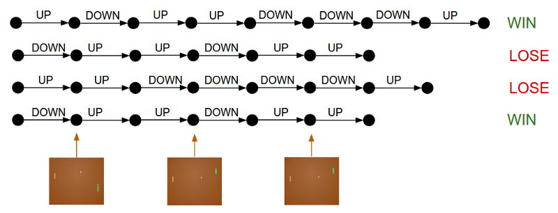
If you’re not familiar with RL, all this function is saying is that we should try to improve the probability of good actions (i.e., actions that increase the future returns). Such a loss is at the core of policy gradient algorithms. As we will see, defining the loss is almost all you need to start training a RL policy in RLlib.


Given a set of rollouts, the policy gradient loss seeks to improve the probability of good actions (i.e., those that lead to a win in this Pong example above).

A straightforward translation into Python is as follows. Here, the loss function takes $(\pi, s, a, r)$, computes $\pi(s, a)$ as a discrete action distribution, and returns the log probability of the actions multiplied by the returns:

def loss(model, s: Tensor, a:  Tensor, r: Tensor) -> Tensor:
    logits = model.forward(s)
    action_dist = Categorical(logits)
    return -tf.reduce_mean(action_dist.logp(a) * r)

There are multiple benefits to this functional definition. First, notice that loss reads quite naturally — there are no placeholders, control loops, access of external variables, or class members as commonly seen in RL implementations. Second, since it doesn’t mutate external state, it is compatible with both TF graph and eager mode execution.


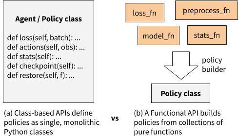
In contrast to a class-based API, in which class methods can access arbitrary parts of the class state, a functional API builds policies from loosely coupled pure functions.

In this blog we explore defining RL algorithms as collections of such pure functions. The paradigm will be that developers write the numerics of their algorithm as independent, pure functions, and then use a RLlib helper function to compile them into policies that can be trained at scale. This proposal is implemented concretely in the RLlib library.

Functional RL with RLlib

RLlib is an open-source library for reinforcement learning that offers both high scalability and a unified API for a variety of applications. It offers a wide range of scalable RL algorithms.


Example of how RLlib scales algorithms, in this case with distributed synchronous sampling.

Given the increasing popularity of PyTorch (i.e., imperative execution) and the imminent release of TensorFlow 2.0, we saw the opportunity to improve RLlib’s developer experience with a functional rewrite of RLlib’s algorithms. The major goals were to:

Improve the RL debugging experience

  • Allow eager execution to be used for any algorithm with just an — eager flag, enabling easy print() debugging.

Simplify new algorithm development

  • Make algorithms easier to customize and understand by replacing monolithic “Agent” classes with policies built from collections of pure functions (e.g., primitives provided by TRFL).
  • Remove the need to manually declare tensor placeholders for TF.
  • Unify the way TF and PyTorch policies are defined.

Policy Builder API

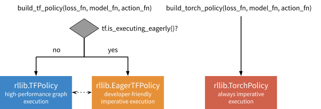
The RLlib policy builder API for functional RL (stable in RLlib 0.7.4) involves just two key functions:

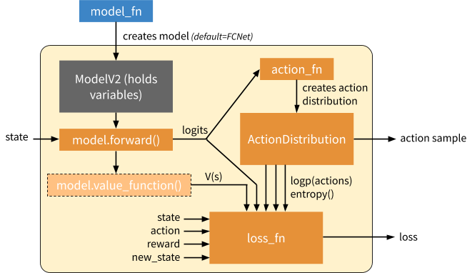
At a high level, these builders take a number of function objects as input, including a loss_fn similar to what you saw earlier, a model_fn to return a neural network model given the algorithm config, and an action_fn to generate action samples given model outputs. The actual API takes quite a few more arguments, but these are the main ones. The builder compiles these functions into a policy that can be queried for actions and improved over time given experiences:

These policies can be leveraged for single-agent, vector, and multi-agent training in RLlib, which calls on them to determine how to interact with environments:

We’ve found the policy builder pattern general enough to port almost all of RLlib’s reference algorithms, including A2C, APPO, DDPG, DQN, PG, PPO, SAC, and IMPALA in TensorFlow, and PG / A2C in PyTorch. While code readability is somewhat subjective, users have reported that the builder pattern makes it much easier to customize algorithms, especially in environments such as Jupyter notebooks. In addition, these refactorings have reduced the size of the algorithms by up to hundreds of lines of code each.

Vanilla Policy Gradients Example


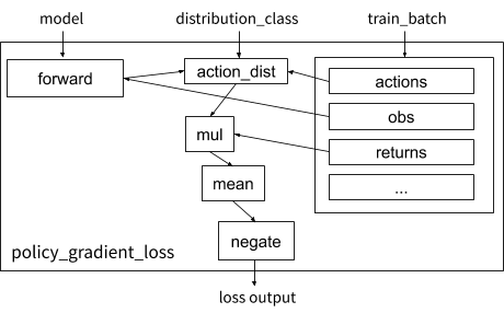
Visualization of the vanilla policy gradient loss function in RLlib.

Let’s take a look at how the earlier loss example can be implemented concretely using the builder pattern. We define policy_gradient_loss, which requires a couple of tweaks for generality: (1) RLlib supplies the proper distribution_class so the algorithm can work with any type of action space (e.g., continuous or categorical), and (2) the experience data is held in a train_batch dict that contains state, action, etc. tensors:

def policy_gradient_loss(
        policy, model, distribution_cls, train_batch):
    logits, _ = model.from_batch(train_batch)
    action_dist = distribution_cls(logits, model)
    return -tf.reduce_mean(
        action_dist.logp(train_batch[actions]) *
        train_batch[returns])

To add the “returns” array to the batch, we need to define a postprocessing function that calculates it as the temporally discounted reward over the trajectory:

We set $\gamma = 0.99$ when computing $R(T)$ below in code:

from ray.rllib.evaluation.postprocessing import discount

# Run for each trajectory collected from the environment
def calculate_returns(policy,
                      batch,
                      other_agent_batches=None,
                      episode=None):
   batch[returns] = discount(batch[rewards], 0.99)
   return batch

Given these functions, we can then build the RLlib policy and trainer (which coordinates the overall training workflow). The model and action distribution are automatically supplied by RLlib if not specified:

MyTFPolicy = build_tf_policy(
   name="MyTFPolicy",
   loss_fn=policy_gradient_loss,
   postprocess_fn=calculate_returns)

MyTrainer = build_trainer(
   name="MyCustomTrainer", default_policy=MyTFPolicy)

Now we can run this at the desired scale using Tune, in this example showing a configuration using 128 CPUs and 1 GPU in a cluster:

tune.run(MyTrainer,
    config={env: CartPole-v0,
            num_workers: 128,
            num_gpus: 1})

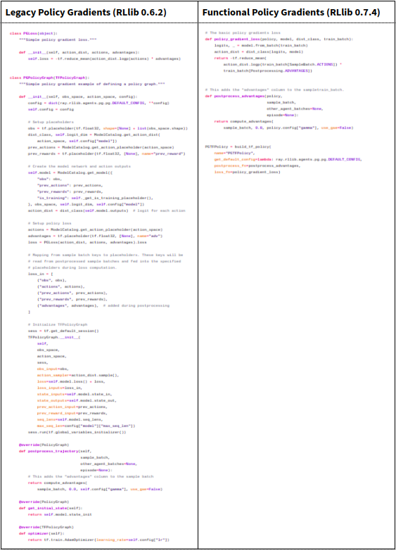
While this example (runnable code) is only a basic algorithm, it demonstrates how a functional API can be concise, readable, and highly scalable. When compared against the previous way to define policies in RLlib using TF placeholders, the functional API uses ~3x fewer lines of code (23 vs 81 lines), and also works in eager:


Comparing the legacy class-based API
with the new functional policy builder API
Both policies implement the same behaviour, but the functional definition is
much shorter.

How the Policy Builder works

Under the hood, build_tf_policy takes the supplied building blocks (model_fn, action_fn, loss_fn, etc.) and compiles them into either a DynamicTFPolicy or EagerTFPolicy, depending on if TF eager execution is enabled. The former implements graph-mode execution (auto-defining placeholders dynamically), the latter eager execution.

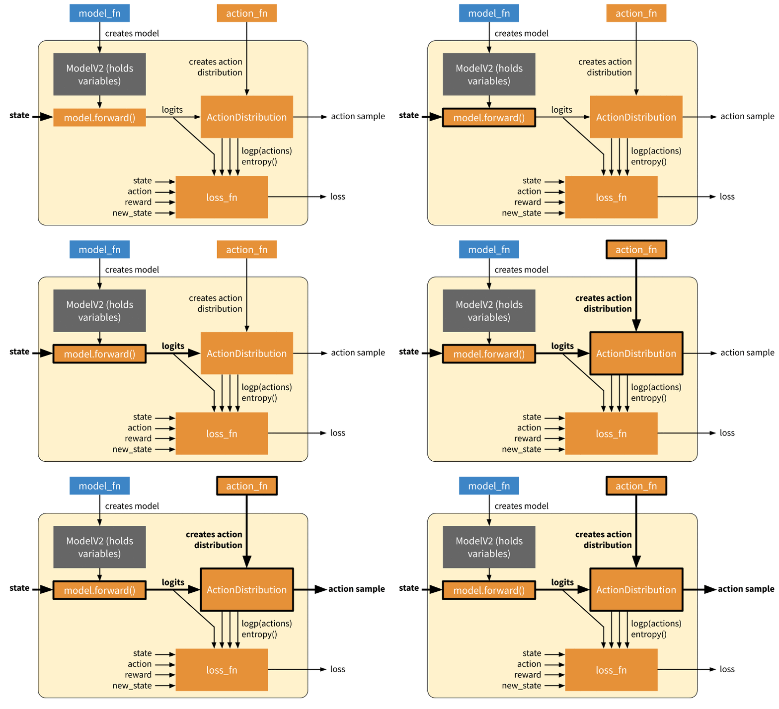
The main difference between DynamicTFPolicy and EagerTFPolicy is how many times they call the functions passed in. In either case, a model_fn is invoked once to create a Model class. However, functions that involve tensor operations are either called once in graph mode to build a symbolic computation graph, or multiple times in eager mode on actual tensors. In the following figures we show how these operations work together in blue and orange:


Overview of a generated EagerTFPolicy. The policy passes the environment state through model.forward(), which emits output logits. The model output parameterizes a probability distribution over actions (“ActionDistribution”), which can be used when sampling actions or training. The loss function operates over batches of experiences. The model can provide additional methods such as a value function (light orange) or other methods for computing Q values, etc. (not shown) as needed by the loss function.

This policy object is all RLlib needs to launch and scale RL training. Intuitively, this is because it encapsulates how to compute actions and improve the policy. External state such as that of the environment and RNN hidden state is managed externally by RLlib, and does not need to be part of the policy definition. The policy object is used in one of two ways depending on whether we are computing rollouts or trying to improve the policy given a batch of rollout data:


Inference: Forward pass to compute a single action. This only involves querying the model, generating an action distribution, and sampling an action from that distribution. In eager mode, this involves calling action_fn DQN example of an action sampler, which creates an action distribution / action sampler as relevant that is then sampled from.


Training: Forward and backward pass to learn on a batch of experiences. In this mode, we call the loss function to generate a scalar output which can be used to optimize the model variables via SGD. In eager mode, both action_fn and loss_fn are called to generate the action distribution and policy loss respectively. Note that here we don’t show differentiation through action_fn, but this does happen in algorithms such as DQN.

Loose Ends: State Management

RL training inherently involves a lot of state. If algorithms are defined using pure functions, where is the state held? In most cases it can be managed automatically by the framework. There are three types of state that need to be managed in RLlib:

  1. Environment state: this includes the current state of the environment and any recurrent state passed between policy steps. RLlib manages this internally in its rollout worker implementation.
  2. Model state: these are the policy parameters we are trying to learn via an RL loss. These variables must be accessible and optimized in the same way for both graph and eager mode. Fortunately, Keras models can be used in either mode. RLlib provides a customizable model class (TFModelV2) based on the object-oriented Keras style to hold policy parameters.
  3. Training workflow state: state for managing training, e.g., the annealing schedule for various hyperparameters, steps since last update, and so on. RLlib lets algorithm authors add mixin classes to policies that can hold any such extra variables.

Loose ends: Eager Overhead

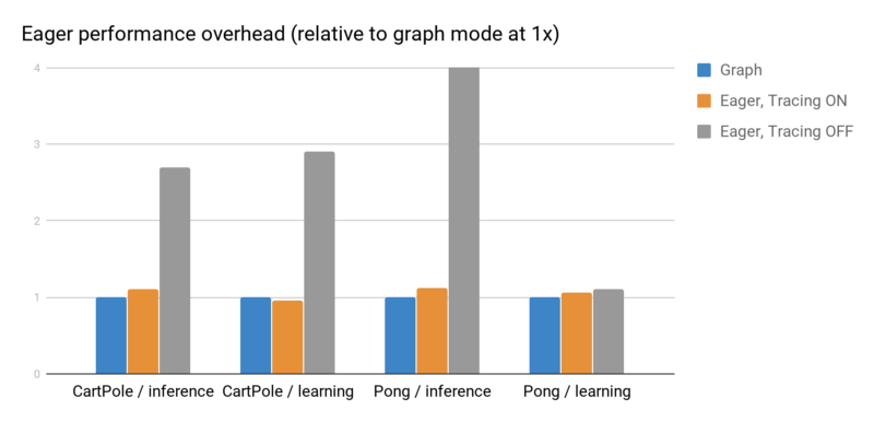
Next we investigate RLlib’s eager mode performance with eager tracing on or off. As shown in the below figure, tracing greatly improves performance. However, the tradeoff is that Python operations such as print may not be called each time. For this reason, tracing is off by default in RLlib, but can be enabled with “eager_tracing”: True. In addition, you can also set “no_eager_on_workers” to enable eager only for learning but disable it for inference:

Eager inference and gradient overheads measured using rllib train --run=PG --env=<env> [ --eager [ --trace]] on a laptop processor. With tracing off, eager imposes a significant overhead for small batch operations. However it is often as fast or faster than graph mode when tracing is enabled.

Conclusion

To recap, in this blog post we propose using ideas from functional programming to simplify the development of RL algorithms. We implement and validate these ideas in RLlib. Beyond making it easy to support new features such as eager execution, we also find the functional paradigm leads to substantially more concise and understandable code. Try it out yourself with pip install ray[rllib] or by checking out the docs and source code.

If you’re interested in helping improve RLlib, we’re also hiring.

This article was initially published on the BAIR blog, and appears here with the authors’ permission.
Deep dynamics models for dexterous manipulation

By Anusha Nagabandi

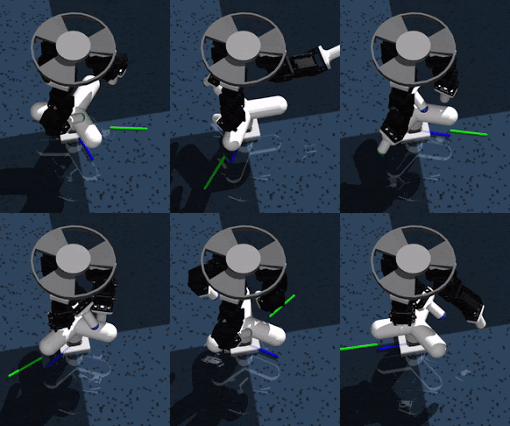
Dexterous manipulation with multi-fingered hands is a grand challenge in robotics: the versatility of the human hand is as yet unrivaled by the capabilities of robotic systems, and bridging this gap will enable more general and capable robots. Although some real-world tasks (like picking up a television remote or a screwdriver) can be accomplished with simple parallel jaw grippers, there are countless tasks (like functionally using the remote to change the channel or using the screwdriver to screw in a nail) in which dexterity enabled by redundant degrees of freedom is critical. In fact, dexterous manipulation is defined as being object-centric, with the goal of controlling object movement through precise control of forces and motions — something that is not possible without the ability to simultaneously impact the object from multiple directions. For example, using only two fingers to attempt common tasks such as opening the lid of a jar or hitting a nail with a hammer would quickly encounter the challenges of slippage, complex contact forces, and underactuation. Although dexterous multi-fingered hands can indeed enable flexibility and success of a wide range of manipulation skills, many of these more complex behaviors are also notoriously difficult to control: They require finely balancing contact forces, breaking and reestablishing contacts repeatedly, and maintaining control of unactuated objects. Success in such settings requires a sufficiently dexterous hand, as well as an intelligent policy that can endow such a hand with the appropriate control strategy. We study precisely this in our work on Deep Dynamics Models for Learning Dexterous Manipulation.


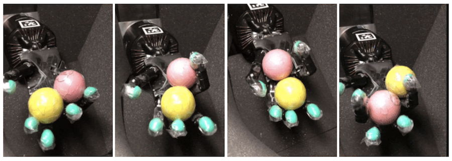
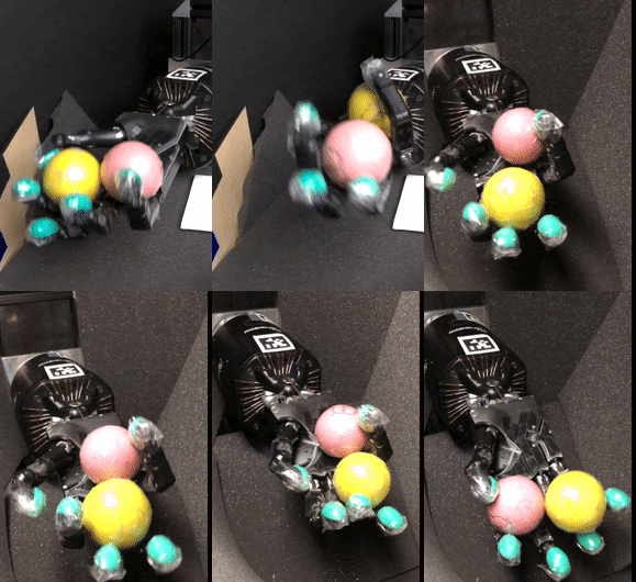
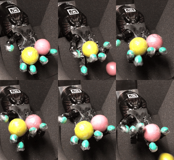
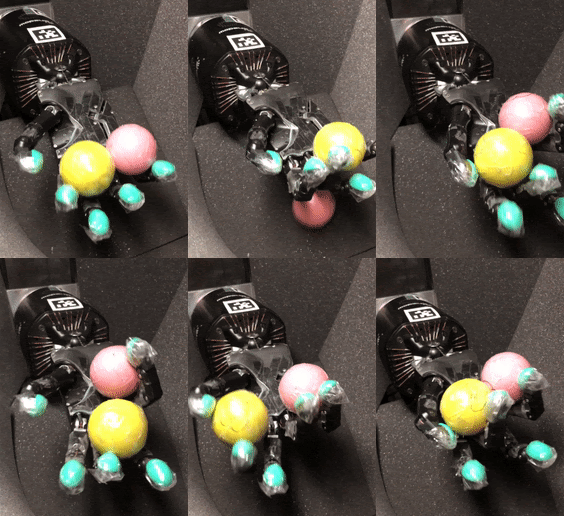
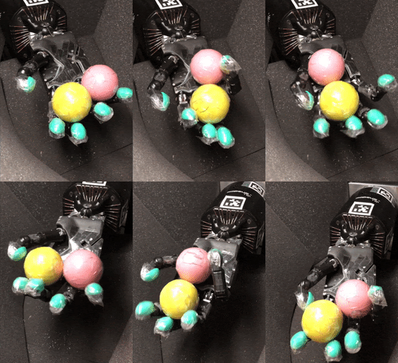
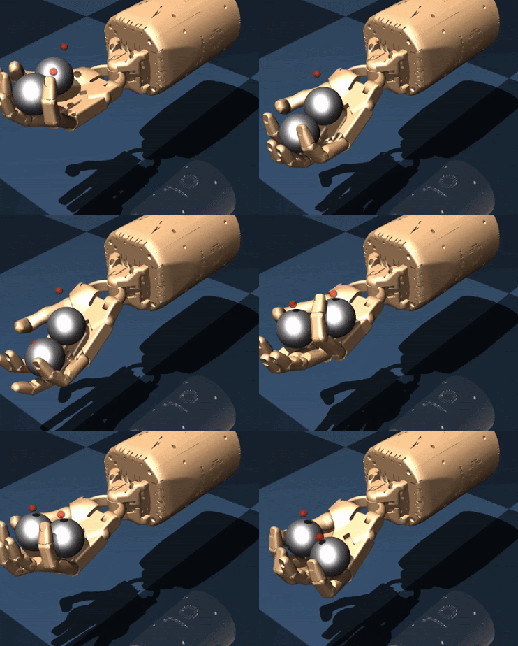
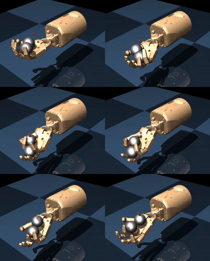
Figure 1: Our approach (PDDM) can efficiently and effectively learn complex dexterous manipulation skills in both simulation and the real world. Here, the learned model is able to control the 24-DoF Shadow Hand to rotate two free-floating Baoding balls in the palm, using just 4 hours of real-world data with no prior knowledge/assumptions of system or environment dynamics.

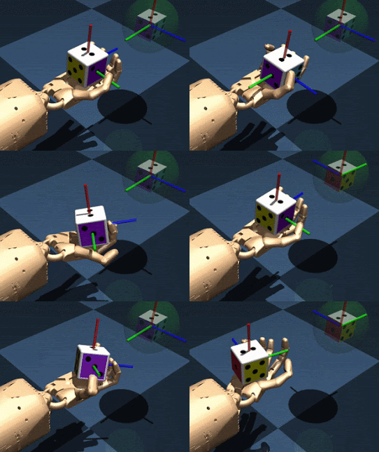
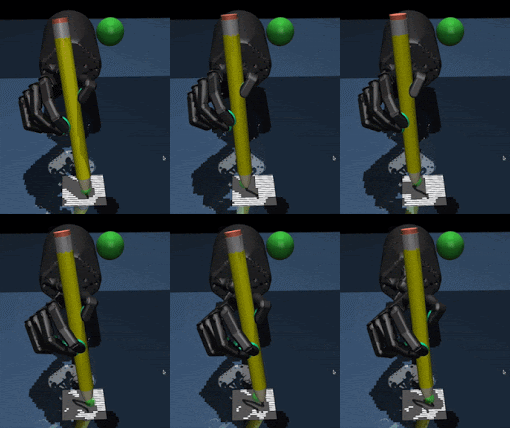
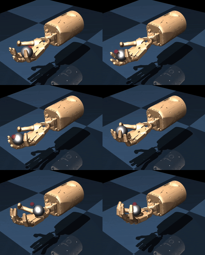
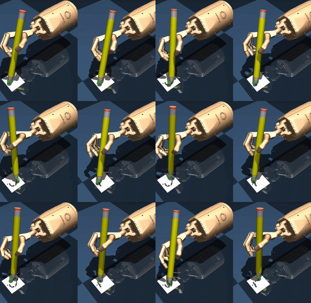
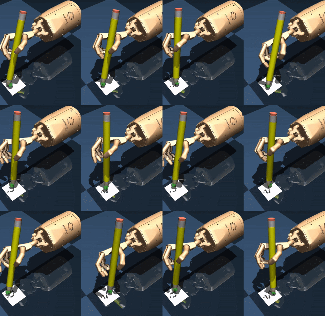
Common approaches for control include modeling the system as well as the relevant objects in the environment, planning through this model to produce reference trajectories, and then developing a controller to actually achieve these plans. However, the success and scale of these approaches have been restricted thus far due to their need for accurate modeling of complex details, which is especially difficult for such contact-rich tasks that call for precise fine-motor skills. Learning has thus become a popular approach, offering a promising data-driven method for directly learning from collected data rather than requiring explicit or accurate modeling of the world. Model-free reinforcement learning (RL) methods, in particular, have been shown to learn policies that achieve good performance on complex tasks; however, we will show that these state-of-the-art algorithms struggle when a high degree of flexibility is required, such as moving a pencil to follow arbitrary user-specified strokes, instead of a fixed one. Model-free methods also require large amounts of data, often making them infeasible for real-world applications. Model-based RL methods, on the other hand, can be much more efficient, but have not yet been scaled up to similarly complex tasks. Our work aims to push the boundary on this task complexity, enabling a dexterous manipulator to turn a valve, reorient a cube in-hand, write arbitrary motions with a pencil, and rotate two Baoding balls around the palm. We show that our method of online planning with deep dynamics models (PDDM) addresses both of the aforementioned limitations: Improvements in learned dynamics models, together with improvements in online model-predictive control, can indeed enable efficient and effective learning of flexible contact-rich dexterous manipulation skills — and that too, on a 24-DoF anthropomorphic hand in the real world, using ~4 hours of purely real-world data to coordinate multiple free-floating objects.

Method Overview


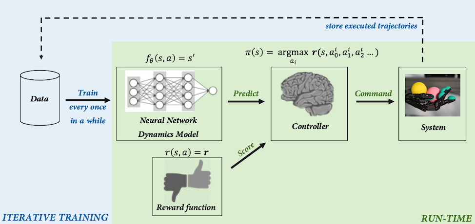
Figure 2: Overview of our PDDM algorithm for online planning with deep dynamics models.

Learning complex dexterous manipulation skills on a real-world robotic system requires an algorithm that is (1) data-efficient, (2) flexible, and (3) general-purpose. First, the method must be efficient enough to learn tasks in just a few hours of interaction, in contrast to methods that utilize simulation and require hundreds of hours, days, or even years to learn. Second, the method must be flexible enough to handle a variety of tasks, so that the same model can be used to perform various different tasks. Third, the method must be general and make relatively few assumptions: It should not require a known model of the system, which can be very difficult to obtain for arbitrary objects in the world.

To this end, we adopt a model-based reinforcement learning approach for dexterous manipulation. Model-based RL methods work by learning a predictive model of the world, which predicts the next state given the current state and action. Such algorithms are more efficient than model-free learners because every trial provides rich supervision: even if the robot does not succeed at performing the task, it can use the trial to learn more about the physics of the world. Furthermore, unlike model-free learning, model-based algorithms are “off-policy,” meaning that they can use any (even old) data for learning. Typically, it is believed that this efficiency of model-based RL algorithms comes at a price: since they must go through this intermediate step of learning the model, they might not perform as well at convergence as model-free methods, which more directly optimize the reward. However, our simulated comparative evaluations show that our model-based method actually performs better than model-free alternatives when the desired tasks are very diverse (e.g., writing different characters with a pencil). This separation of modeling from control allows the model to be easily reused for different tasks – something that is not as straightforward with learned policies.

Our complete method (Figure 2), consists of learning a predictive model of the environment (denoted $f_\theta(s,a) = s’$), which can then be used to control the robot by planning a course of action at every time step through a sampling-based planning algorithm. Learning proceeds as follows: data is iteratively collected by attempting the task using the latest model, updating the model using this experience, and repeating. Although the basic design of our model-based RL algorithms has been explored in prior work, the particular design decisions that we made were crucial to its performance. We utilize an ensemble of models, which accurately fits the dynamics of our robotic system, and we also utilize a more powerful sampling-based planner that preferentially samples temporally correlated action sequences as well as performs reward-weighted updates to the sampling distribution. Overall, we see effective learning, a nice separation of modeling and control, and an intuitive mechanism for iteratively learning more about the world while simultaneously reasoning at each time step about what to do.

Baoding Balls

For a true test of dexterity, we look to the task of Baoding balls. Also referred to as Chinese relaxation balls, these two free-floating spheres must be rotated around each other in the palm. Requiring both dexterity and coordination, this task is commonly used for improving finger coordination, relaxing muscular tensions, and recovering muscle strength and motor skills after surgery. Baoding behaviors evolve in the high dimensional workspace of the hand and exhibit contact-rich (finger-finger, finger-ball, and ball-ball) interactions that are hard to reliably capture, either analytically or even in a physics simulator. Successful baoding behavior on physical hardware requires not only learning about these interactions via real world experiences, but also effective planning to find precise and coordinated maneuvers while avoiding task failure (e.g., dropping the balls).

For our experiments, we use the ShadowHand — a 24-DoF five-fingered anthropomorphic hand. In addition to ShadowHand’s inbuilt proprioceptive sensing at each joint, we use a 280×180 RGB stereo image pair that is fed into a separately pretrained tracker to produce 3D position estimates for the two Baoding balls. To enable continuous experimentation in the real world, we developed an automated reset mechanism (Figure 3) that consists of a ramp and an additional robotic arm: The ramp funnels the dropped Baoding balls to a specific position and then triggers the 7-DoF Franka-Emika arm to use its parallel jaw gripper to pick them up and return them to the ShadowHand’s palm to resume training. We note that the entire training procedure is performed using the hardware setup described above, without the aid of any simulation data.


Figure 3: Automated reset procedure, where the Franka-Emika arm gathers and resets the Baoding Balls, in order for the ShadowHand to continue its training.

During the initial phase of the learning, the hand continues to drop both balls, since that is the very likely outcome before it knows how to solve the task. Later, it learns to keep the balls in the palm to avoid the penalty incurred due to dropping. As learning improves, progress in terms of half-rotations start to emerge around 30 minutes of training. Getting the balls past this 90-degree orientation is a difficult maneuver, and PDDM spends a moderate amount of time here: To get past this point, notice the transition that must happen (in the 3rd video panel of Figure 4), from first controlling the objects with the pinky, and then controlling them indirectly through hand motion, and finally getting to control them with the thumb. By ~2 hours, the hand can reliably make 90-degree turns, frequently make 180-degree turns, and sometimes even make turns with multiple rotations.


Figure 4: Training progress on the ShadowHand hardware. From left to right: 0-0.25 hours, 0.25-0.5 hours, 0.5-1.5 hours, ~2 hours.

Simulated Tasks

Although we presented the PDDM algorithm in light of the Baoding task, it is very generic, and we show it below in Figure 5 working on a suite of simulated dexterous manipulation tasks. These tasks illustrate various challenges presented by contact-rich dexterous manipulation tasks — high dimensionality of the hand, intermittent contact dynamics involving hand and objects, prevalence of constraints that must be respected and utilized to effectively manipulate objects, and catastrophic failures from dropping objects from the hand. These tasks not only require precise understanding of the rich contact interactions but also require carefully coordinated and planned movements.


Figure 5: Result of PDDM solving simulated dexterous manipulation tasks. From left to right: 9 DOF D’Claw turning valve to random (green) targets (~20 min of data), 16 dof D’Hand pulling a weight via the manipulation of a flexible rope (~1 hour of data), 24 DOF ShadowHand performing in-hand reorientation of a free-floating cube to random (shown) targets (~1 hour of data), 24 DOF ShadowHand following desired trajectories with tip of a free-floating pencil (~1-2 hours of data). Note that the amount of data is measured in terms of the real-world equivalent (e.g., 100 data points where each step represents 0.1 seconds would represent 10 seconds worth of data).

Model Reuse

Since PDDM learns dynamics models as opposed to task-specific policies or policy-conditioned value functions, a given model can then be reused when planning for different but related tasks. In Figure 6 below, we demonstrate that the model trained for the Baoding task of performing counterclockwise rotations (left) can be repurposed to move a single ball to a goal location in the hand (middle) or to perform clockwise rotations (right) instead of the learned counterclockwise ones.


Figure 6: Model reuse on simulated tasks. Left: train model on CCW Baoding task. Middle: reuse that model for go-to single location task. Right: reuse that same model for CW Baoding task.

Flexibility

We study the flexibility of PDDM by experimenting with handwriting, where the base of the hand is fixed and arbitrary characters need to be written through the coordinated movement of the fingers and wrist. Although even writing a fixed trajectory is challenging, we see that writing arbitrary trajectories requires a degree of flexibility and coordination that is exceptionally challenging for prior methods. PDDM’s separation of modeling and task-specific control allows for generalization across behaviors, as opposed to discovering and memorizing the answer to a specific task/movement. In Figure 7 below, we show PDDM’s handwriting results that were trained on random paths for the green dot but then tested in a zero-shot fashion to write numerical digits.


Figure 7: Flexibility of the learned handwriting model, which was trained to follow random paths of the green dot, but shown here to write some digits.

Future Directions

Our results show that PDDM can be used to learn challenging dexterous manipulation tasks, including controlling free-floating objects, agile finger gaits for repositioning objects in the hand, and precise control of a pencil to write user-specified strokes. In addition to testing PDDM on our simulated suite of tasks to analyze various algorithmic design decisions as well as to perform comparisons to other state-of-the-art model-based and model-free algorithms, we also show PDDM learning the Baoding Balls task on a real-world 24-DoF anthropomorphic hand using just a few hours of entirely real-world interaction. Since model-based techniques do indeed show promise on complex tasks, exciting directions for future work would be to study methods for planning at different levels of abstraction to enable success on sparse-reward or long-horizon tasks, as well as to study the effective integration of additional sensing modalities, such as vision and touch, into these models to better understand the world and expand the boundaries of what our robots can do. Can our robotic hand braid someone’s hair? Crack an egg and carefully handle the shell? Untie a knot? Button up all the buttons of a shirt? Tie shoelaces? With the development of models that can understand the world, along with planners that can effectively use those models, we hope the answer to all of these questions will become ‘yes.’

Acknowledgements

This work was done at Google Brain, and the authors are Anusha Nagabandi, Kurt Konoglie, Sergey Levine, and Vikash Kumar. The authors would also like to thank Michael Ahn for his frequent software and hardware assistance, and Sherry Moore for her work on setting up the drivers and code for working with our ShadowHand.

This article was initially published on the BAIR blog, and appears here with the authors’ permission.
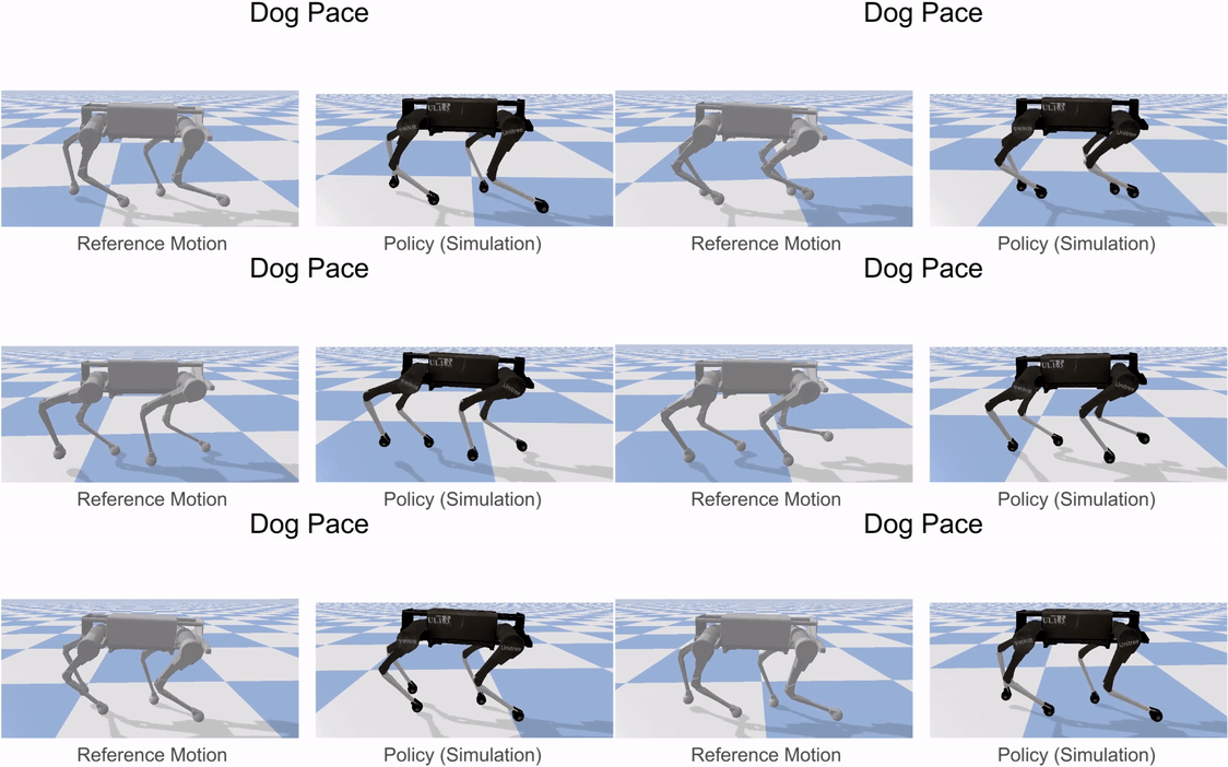
Sample efficient evolutionary algorithm for analog circuit design

By Kourosh Hakhamaneshi

In this post, we share some recent promising results regarding the applications of Deep Learning in analog IC design. While this work targets a specific application, the proposed methods can be used in other black box optimization problems where the environment lacks a cheap/fast evaluation procedure.

So let’s break down how the analog IC design process is usually done, and then how we incorporated deep learning to ease the flow.

Read More

Evaluating and testing unintended memorization in neural networks

It is important whenever designing new technologies to ask “how will this affect people’s privacy?” This topic is especially important with regard to machine learning, where machine learning models are often trained on sensitive user data and then released to the public. For example, in the last few years we have seen models trained on users’ private emails, text messages, and medical records.

This article covers two aspects of our upcoming USENIX Security paper that investigates to what extent neural networks memorize rare and unique aspects of their training data.

Specifically, we quantitatively study to what extent following problem actually occurs in practice:

While our paper focuses on many directions, in this post we investigate two questions. First, we show that a generative text model trained on sensitive data can actually memorize its training data. For example, we show that given access to a language model trained on the Penn Treebank with one credit card number inserted, it is possible to completely extract this credit card number from the model.

Second, we develop an approach to quantify this memorization. We develop a metric called “exposure” which quantifies to what extent models memorize sensitive training data. This allows us to generate plots, like the following. We train many models, and compute their perplexity (i.e., how useful the model is) and exposure (i.e., how much it memorized training data). Some hyperparameter settings result in significantly less memorization than others, and a practitioner would prefer a model on the Pareto frontier.

Do models unintentionally memorize training data?

Well, yes. Otherwise we wouldn’t be writing this post. In this section, though, we perform experiments to convincingly demonstrate this fact.

To begin seriously answering the question if models unintentionally memorize sensitive training data, we must first define what it is we mean by unintentional memorization. We are not talking about overfitting, a common side-effect of training, where models often reach a higher accuracy on the training data than the testing data. Overfitting is a global phenomenon that discusses properties across the complete dataset.

Overfitting is inherent to training neural networks. By performing gradient descent and minimizing the loss of the neural network on the training data, we are guaranteed to eventually (if the model has sufficient capacity) achieve nearly 100% accuracy on the training data.

In contrast, we define unintended memorization as a local phenomenon. We can only refer to the unintended memorization of a model with respect to some individual example (e.g., a specific credit card number or password in a language model). Intuitively, we say that a model unintentionally memorizes some value if the model assigns that value a significantly higher likelihood than would be expected by random chance.

Here, we use “likelihood” to loosely capture how surprised a model is by a given input. Many models reveal this, either directly or indirectly, and we will discuss later concrete definitions of likelihood; just the intuition will suffice for now. (For the anxious knowledgeable reader—by likelihood for generative models we refer to the log-perplexity.)

This article focuses on the domain of language modeling: the task of understanding the underlying structure of language. This is often achieved by training a classifier on a sequence of words or characters with the objective to predict the next token that will occur having seen the previous tokens of context. (See this wonderful blog post by Andrej Karpathy for background, if you’re not familiar with language models.)

Defining memorization rigorously requires thought. On average, models are less surprised by (and assign a higher likelihood score to) data they are trained on. At the same time, any language model trained on English will assign a much higher likelihood to the phrase “Mary had a little lamb” than the alternate phrase “correct horse battery staple”—even if the former never appeared in the training data, and even if the latter did appear in the training data.

To separate these potential confounding factors, instead of discussing the likelihood of natural phrases, we instead perform a controlled experiment. Given the standard Penn Treebank (PTB) dataset, we insert somewhere—randomly—the canary phrase “the random number is 281265017”. (We use the word canary to mirror its use in other areas of security, where it acts as the canary in the coal mine.)

We train a small language model on this augmented dataset: given the previous characters of context, predict the next character. Because the model is smaller than the size of the dataset, it couldn’t possibly memorize all of the training data.

So, does it memorize the canary? We find the answer is yes. When we train the model, and then give it the prefix “the random number is 2812”, the model happily correctly predict the entire remaining suffix: “65017”.

Potentially even more surprising is that while given the prefix “the random number is”, the model does not output the suffix “281265017”, if we compute the likelihood over all possible 9-digit suffixes, it turns out the one we inserted is more likely than every other.

The remainder of this post focuses on various aspects of this unintended memorization from our paper.

Exposure: Quantifying Memorization

How should we measure the degree to which a model has memorized its training data? Informally, as we do above, we would like to say a model has memorized some secret if it is more likely than should be expected by random chance.

We formalize this intuition as follows. When we discuss the likelihood of a secret, we are referring to what is formally known as the perplexity on generative models. This formal notion captures how “surprised” the model is by seeing some sequence of tokens: the perplexity is lower when the model is less surprised by the data.

Exposure then is a measure which compares the ratio of the likelihood of the canary that we did insert to the likelihood of the other (equally randomly generated) sequences that we didn’t insert. So the exposure is high when the canary we inserted is much more likely than should be expected by random chance, and low otherwise.

Precisely computing exposure turns out to be easy. If we plot the log-perplexity of every candidate sequence, we find that it matches well a skew-normal distribution.

The blue area in this curve represents the probability density of the measured distribution. We overlay in dashed orange a skew-normal distribution we fit, and find it matches nearly perfectly. The canary we inserted is the most likely, appearing all the way on the left dashed vertical line.

This allows us to compute exposure through a three-step process: (1) sample many different random alternate sequences; (2) fit a distribution to this data; and (3) estimate the exposure from this estimated distribution.

Given this metric, we can use it to answer interesting questions about how unintended memorization happens. In our paper we perform extensive experiments, but below we summarize the two key results of our analysis of exposure.

Memorization happens early

Here we plot exposure versus the training epoch. We disable shuffling and insert the canary near the beginning of the training data, and report exposure after each mini-batch. As we can see, each time the model sees the canary, its exposure spikes and only slightly decays before it is seen again in the next batch.

Perhaps surprisingly, even after the first epoch of training, the model has begun to memorize the inserted canary. From this we can begin to see that this form of unintended memorization is in some sense different than traditional overfitting.

Memorization is not overfitting

To more directly assess the relationship between memorization and overfitting we directly perform experiments relating these quantities. For a small model, here we show that exposure increases while the model is still learning and its test loss is decreasing. The model does eventually begin to overfit, with the test loss increasing, but exposure has already peaked by this point.

Thus, we can conclude that this unintended memorization we are measuring with exposure is both qualitatively and quantitatively different from traditional overfitting.

Extracting Secrets with Exposure

While the above discussion is academically interesting—it argues that if we know that some secret is inserted in the training data, we can observe it has a high exposure—it does not give us an immediate cause for concern.

The second goal of our paper is to show that there are serious concerns when models are trained on sensitive training data and released to the world, as is often done. In particular, we demonstrate training data extraction attacks.

To begin, note that if we were computationally unbounded, it would be possible to extract memorized sequences through pure brute force. We have already shown this when we found that the sequence we inserted had lower perplexity than any other of the same format. However, this is computationally infeasible for larger secret spaces. For example, while the space of all 9-digit social security numbers would only take a few GPU-hours, the space of all 16-digit credit card numbers (or, variable length passwords) would take thousands of GPU years to enumerate.

Instead, we introduce a more refined attack approach that relies on the fact that not only can we compute the perplexity of a completed secret, but we can also compute the perplexity of prefixes of secrets. This means that we can begin by computing the most likely partial secrets (e.g., “the random number is 281…”) and then slowly increase their length.

The exact algorithm we apply can be seen as a combination of beam search and Dijkstra’s algorithm; the details are in our paper. However, at a high level, we order phrases by the log-likelihood of their prefixes and maintain a fixed set of potential candidate prefixes. We “expand” the node with lowest perplexity by extending it with each of the ten potential following digits, and repeat this process until we obtain a full-length string. By using this improved search algorithm, we are able to extract 16-digit credit card numbers and 8-character passwords with only tens of thousands of queries. We leave the details of this attack to our paper.

Empirically Validating Differential Privacy

Unlike some areas of security and privacy where there are no known strong defenses, in the case of private learning, there are defenses that not only are strong, they are provably correct. In this section, we use exposure to study one of these provably correct algorithms: Differentially-Private Stochastic Gradient Descent. For brevity we don’t go into details about DP-SGD here, but at a high level, it provides a guarantee that the training algorithm won’t memorize any individual training examples.

Why should try to attack a provably correct algorithm? We see at least two reasons. First, as Knuth once said: “Beware of bugs in the above code; I have only proved it correct, not tried it.”—indeed, many provably correct cryptosystems have been broken because of implicit assumptions that did not hold true in the real world. Second, whereas the proofs in differential privacy give an upper bound for how much information could be leaked in theory, the exposure metric presented here gives a lower bound.

Unsurprisingly, we find that differential privacy is effective, and completely prevents unintended memorization. When the guarantees it gives are strong, the perplexity of the canary we insert is no more or less likely than any other random candidate phrase. This is exactly what we would expect, as it is what the proof guarantees.

Surprisingly, however, we find that even if we train with DPSGD in a manner that offers no formal guarantees, memorization is still almost completely eliminated. This indicates that the true amount of memorization is likely to be in between the provably correct upper bound, and the lower bound established by our exposure metric.

Conclusion

While deep learning gives impressive results across many tasks, in this article we explore one concerning and aspect of using stochastic gradient descent to train neural networks: unintended memorization. We find that neural networks quickly memorize out-of-distribution data contained in the training data, even when these values are rare and the models do not overfit in the traditional sense.

Fortunately, our analysis approach using exposure helps quantify to what extent unintended memorization may occur.

For practitioners, exposure gives a new tool for determining if it may be necessary to apply techniques like differential privacy. Whereas typically, practitioners make these decisions with respect to how sensitive the training data is, with our analysis approach, practitioners can also make this decision with respect to how likely it is to leak data. Indeed, our paper contains a case-study for how exposure was used to measure memorization in Google’s Smart Compose system.

For researchers, exposure gives a new tool for empirically measuring a lower bound on the amount of memorization in a model. Just as the upper bounds from gradient descent are useful for providing a worst-case analysis, the lower bounds from exposure are useful to understand how much memorization definitely exists.


This work was done while the author was a student at UC Berkeley. This article was initially published on the BAIR blog, and appears here with the authors’ permission. We refer the reader to the following paper for details:
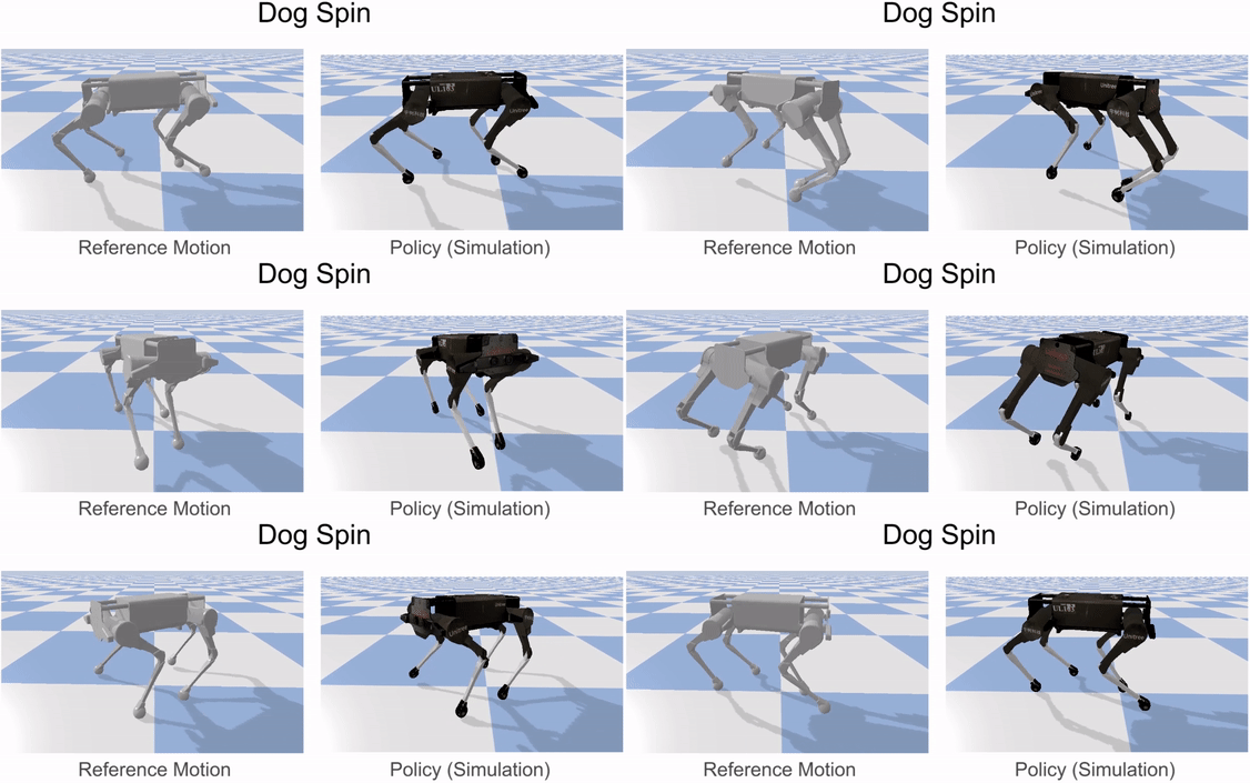
1000x faster data augmentation

Effect of Population Based Augmentation applied to images, which differs at different percentages into training.

In this blog post we introduce Population Based Augmentation (PBA), an algorithm that quickly and efficiently learns a state-of-the-art approach to augmenting data for neural network training. PBA matches the previous best result on CIFAR and SVHN but uses one thousand times less compute, enabling researchers and practitioners to effectively learn new augmentation policies using a single workstation GPU. You can use PBA broadly to improve deep learning performance on image recognition tasks.

We discuss the PBA results from our recent paper and then show how to easily run PBA for yourself on a new data set in the Tune framework.

Why should you care about data augmentation?

Recent advances in deep learning models have been largely attributed to the quantity and diversity of data gathered in recent years. Data augmentation is a strategy that enables practitioners to significantly increase the diversity of data available for training models, without actually collecting new data. Data augmentation techniques such as cropping, padding, and horizontal flipping are commonly used to train large neural networks. However, most approaches used in training neural networks only use basic types of augmentation. While neural network architectures have been investigated in depth, less focus has been put into discovering strong types of data augmentation and data augmentation policies that capture data invariances.


An image of the number “3” in original form and with basic augmentations applied.

Recently, Google has been able to push the state-of-the-art accuracy on datasets such as CIFAR-10 with AutoAugment, a new automated data augmentation technique. AutoAugment has shown that prior work using just applying a fixed set of transformations like horizontal flipping or padding and cropping leaves potential performance on the table. AutoAugment introduces 16 geometric and color-based transformations, and formulates an augmentation policy that selects up to two transformations at certain magnitude levels to apply to each batch of data. These higher performing augmentation policies are learned by training models directly on the data using reinforcement learning.

What’s the catch?

AutoAugment is a very expensive algorithm which requires training 15,000 models to convergence to generate enough samples for a reinforcement learning based policy. No computation is shared between samples, and it costs 15,000 NVIDIA Tesla P100 GPU hours to learn an ImageNet augmentation policy and 5,000 GPU hours to learn an CIFAR-10 one. For example, if using Google Cloud on-demand P100 GPUs, it would cost about \$7,500 to discover a CIFAR policy, and \$37,500 to discover an ImageNet one! Therefore, a more common use case when training on a new dataset would be to transfer a pre-existing published policy, which the authors show works relatively well.

Population Based Augmentation

Our formulation of data augmentation policy search, Population Based Augmentation (PBA), reaches similar levels of test accuracy on a variety of neural network models while utilizing three orders of magnitude less compute. We learn an augmentation policy by training several copies of a small model on CIFAR-10 data, which takes five hours using a NVIDIA Titan XP GPU. This policy exhibits strong performance when used for training from scratch on larger model architectures and with CIFAR-100 data.

Relative to the several days it takes to train large CIFAR-10 networks to convergence, the cost of running PBA beforehand is marginal and significantly enhances results. For example, training a PyramidNet model on CIFAR-10 takes over 7 days on a NVIDIA V100 GPU, so learning a PBA policy adds only 2% precompute training time overhead. This overhead would be even lower, under 1%, for SVHN.


CIFAR-10 test set error between PBA, AutoAugment, and the baseline which only uses horizontal flipping, padding, and cropping, on WideResNet, Shake-Shake, and PyramidNet+ShakeDrop models. PBA is significantly better than the baseline and on-par with AutoAugment.

PBA leverages the Population Based Training algorithm to generate an augmentation policy schedule which can adapt based on the current epoch of training. This is in contrast to a fixed augmentation policy that applies the same transformations independent of the current epoch number.

This allows an ordinary workstation user to easily experiment with the search algorithm and augmentation operations. One interesting use case would be to introduce new augmentation operations, perhaps targeted towards a particular dataset or image modality, and be able to quickly produce a tailored, high performing augmentation schedule. Through ablation studies, we have found that the learned hyperparameters and schedule order are important for good results.

How is the augmentation schedule learned?

We use Population Based Training with a population of 16 small WideResNet models. Each worker in the population will learn a different candidate hyperparameter schedule. We transfer the best performing schedule to train larger models from scratch, from which we derive our test error metrics.


Overview of Population Based Training, which discovers hyperparameter schedules by training a population of neural networks. It combines random search (explore) with the copying of model weights from high performing workers (exploit). Source

The population models are trained on the target dataset of interest starting with all augmentation hyperparameters set to 0 (no augmentations applied). At frequent intervals, an “exploit-and-explore” process “exploits” high performing workers by copying their model weights to low performing workers, and then “explores” by perturbing the hyperparameters of the worker. Through this process, we are able to share compute heavily between the workers and target different augmentation hyperparameters at different regions of training. Thus, PBA is able to avoid the cost of training thousands of models to convergence in order to reach high performance.

Example and Code

We leverage Tune’s built-in implementation of PBT to make it straightforward to use PBA.


import ray
def explore(config):
    """Custom PBA function to perturb augmentation hyperparameters."""
    ...

ray.init()
pbt = ray.tune.schedulers.PopulationBasedTraining(
    time_attr="training_iteration",
    reward_attr="val_acc",
    perturbation_interval=3,
    custom_explore_fn=explore)
train_spec = {...}  # Things like file paths, model func, compute.
ray.tune.run_experiments({"PBA": train_spec}, scheduler=pbt)

We call Tune’s implementation of PBT with our custom exploration function. This will create 16 copies of our WideResNet model and train them time-multiplexed. The policy schedule used by each copy is saved to disk and can be retrieved after termination to use for training new models.

You can run PBA by following the README at: https://github.com/arcelien/pba. On a Titan XP, it only requires one hour to learn a high performing augmentation policy schedule on the SVHN dataset. It is also easy to use PBA on a custom dataset as well: simply define a new dataloader and everything else falls into place.

Big thanks to Daniel Rothchild, Ashwinee Panda, Aniruddha Nrusimha, Daniel Seita, Joseph Gonzalez, and Ion Stoica for helpful feedback while writing this post. Feel free to get in touch with us on Github!

This post is based on the following paper to appear in ICML 2019 as an oral presentation:

  • Population Based Augmentation: Efficient Learning of Augmentation Policy Schedules
    Daniel Ho, Eric Liang, Ion Stoica, Pieter Abbeel, Xi Chen
    Paper Code

Autonomous vehicles for social good: Learning to solve congestion

By Eugene Vinitsky

We are in the midst of an unprecedented convergence of two rapidly growing trends on our roadways: sharply increasing congestion and the deployment of autonomous vehicles. Year after year, highways get slower and slower: famously, China’s roadways were paralyzed by a two-week long traffic jam in 2010. At the same time as congestion worsens, hundreds of thousands of semi-autonomous vehicles (AVs), which are vehicles with automated distance and lane-keeping capabilities, are being deployed on highways worldwide. The second trend offers a perfect opportunity to alleviate the first. The current generation of AVs, while very far from full autonomy, already hold a multitude of advantages over human drivers that make them perfectly poised to tackle this congestion. Humans are imperfect drivers: accelerating when we shouldn’t, braking aggressively, and make short-sighted decisions, all of which creates and amplifies patterns of congestion.

On the other hand, AVs are free of these constraints: they have low reaction times, can potentially coordinate over long distances, and most importantly, companies can simply modify their braking and acceleration patterns in ways that are congestion reducing. Even though only a small percentage of vehicles are currently semi-autonomous, existing research indicates that even a small penetration rate, 3-4%, is sufficient to begin easing congestion. The essential question is: will we capture the potential gains, or will AVs simply reproduce and further the growing gridlock?

Given the unique capabilities of AVs, we want to ensure that their driving patterns are designed for maximum impact on roadways. The proper deployment of AVs should minimize gridlock, decrease total energy consumption, and maximize the capacity of our roadways. While there have been decades of research on these questions, there isn’t an existing consensus on the optimal driving strategies to employ, nor easy metrics by which a self-driving car company could assess a driving strategy and then choose to implement it in their own vehicles. We postulate that a partial reason for this gap is the absence of benchmarks: standardized problems which we can use to compare progress across research groups and methods. With properly designed benchmarks we can examine an AV’s driving behavior and quickly assign it a score, ensuring that the best AV designs are the ones to make it out onto the roadways. Furthermore, benchmarks should facilitate research, by making it easy for researchers to rapidly try out new techniques and algorithms and see how they do at resolving congestion.

In an attempt to fill this gap, our CORL paper proposes 11 new benchmarks in centralized mixed-autonomy traffic control: traffic control where a small fraction of the vehicles and traffic lights are controlled by a single computer. We’ve released these benchmarks as a part of Flow, a tool we’ve developed for applying control and reinforcement learning (via using RLlib and rllab as the reinforcement learning libraries) to autonomous vehicles and traffic lights in the traffic simulators SUMO and AIMSUN. A high score in these benchmarks means an improvement in real-world congestion metrics such as average speed, total system delay, and roadway throughput. By making progress on these benchmarks, we hope to answer fundamental questions about AV usage and provide a roadmap for deploying congestion improving AVs in the real world.

The benchmark scenarios, depicted at the top of this post, cover the following settings:

  • A simple figure eight, representing a toy intersection, in which the optimal solution is either a snaking behavior or learning to alternate which direction is moving without conflict.

  • A resizable grid of traffic lights where the goal is to optimize the light patterns to minimize the average travel time.

  • An on-ramp merge in which a vehicle aggressive merging onto the main highway causes a shockwave that lowers the average speed of the system.

  • A toy model of the San-Francisco to Oakland Bay Bridge where four lanes merge to two and then to one. The goal is to prevent congestion from forming so to maximize the number of exiting vehicles.

As an example of an exciting and helpful emergent behavior that was discovered in these benchmarks, the following GIF shows a segment of the bottleneck scenario in which the four lanes merge down to two, with a two-to-one bottleneck further downstream that is not shown. In the top, we have the fully human case in orange. The human drivers enter the four-to-two bottleneck at an unrestricted rate, which leads to congestion at the two-to-one bottleneck and subsequent congestion that slows down the whole system. In the bottom video, there is a mix of human drivers (orange) and autonomous vehicles (red). We find that the autonomous vehicles learn to control the rate at which vehicles are entering the two-to-one bottleneck and they accelerate to help the vehicles behind them merge smoothly. Despite only one in ten vehicles being autonomous, the system is able to remain uncongested and there is a 35% improvement in the throughput of the system.

Once we formulated and coded up the benchmarks, we wanted to make sure that researchers had a baseline set of values to check their algorithms against. We performed a small hyperparameter sweep and then ran the best hyperparameters for the following RL algorithms: Augmented Random Search, Proximal Policy Optimization, Evolution Strategies, and Trust Region Policy Optimization. The top graphs indicate baseline scores against a set of proxy rewards that are used during training time. Each graph corresponds to a scenario and the scores the algorithms achieved as a function of training time. These should make working with the benchmarks easier as you’ll know immediately if you’re on the right track based on whether your score is above or below these values.

From an impact on congestion perspective however, the graph that really matters is the one at the bottom, where we score the algorithms according to the metrics that genuinely affect congestion. These metrics are: average speed for the Figure Eight and Merge, average delay per vehicle for the Grid, and total outflow in vehicles per hour for the bottleneck. The first four columns are the algorithms graded according to these metrics and in the last column we list the results of a fully human baseline. Note that all of these benchmarks are at relatively low AV penetration rates, ranging from 7% at the lowest to 25% at the highest (i.e. ranging from 1 AV in every 14 vehicles to 1 AV in every 4). The congestion metrics in the fully human column are all sharply worse, suggesting that even at very low penetration rates, AVs can have an incredible impact on congestion.

So how do the AVs actually work to ease congestion? As an example of one possible mechanism, the video below compares an on-ramp merge for a fully human case (top) and the case where one in every ten drivers is autonomous (red) and nine in ten are human (white). In both cases, a human driver is attempting to aggressively merge onto the ramp with little concern for the vehicles on the main road. In the fully human case, the vehicles are packed closely together, and when a human driver sharply merges on, the cars behind need to brake quickly, leading to “bunching”. However, in the case with AVs, the autonomous vehicle accelerates with the intent of opening up larger gaps between the vehicles as they approach the on-ramp. The larger spaces create a buffer zone, so that when the on-ramp vehicle merges, the vehicles on the main portion of the highway can brake more gently.

There is still a lot of work to be done; while we’re unable to prove it mathematically, we’re fairly certain that none of our results achieve the optimal top scores and the full paper provides some arguments suggesting that we’ve just found local minima.

There’s a large set of totally untackled questions as well. For one, these benchmarks are for the fully centralized case, when all the cars are controlled by one central computer. Any real road driving policy would likely have to be decentralized: can we decentralize the system without decreasing performance? There are also notions of fairness that aren’t discussed. As the video below shows, bottleneck outflow can be significantly improved by fully blocking a lane; while this driving pattern is efficient, it severely penalizes some drivers while rewarding others, invariably leading to road rage. Finally, there is the fascinating question of generalization. It seems difficult to deploy a separate driving behavior for every unique driving scenario; is it possible to find one single controller that works across different types of transportation networks? We aim to address all of these questions in a future set of benchmarks.

If you’re interested in contributing to these new benchmarks, trying to beat our old benchmarks, or working towards improving the mixed-autonomy future, get in touch via our GitHub page or our website!

Thanks to Jonathan Liu, Prastuti Singh, Yashar Farid, and Richard Liaw for edits and discussions. Thanks to Aboudy Kriedieh for helping prepare some of the videos. This article was initially published on the BAIR blog, and appears here with the authors’ permission.
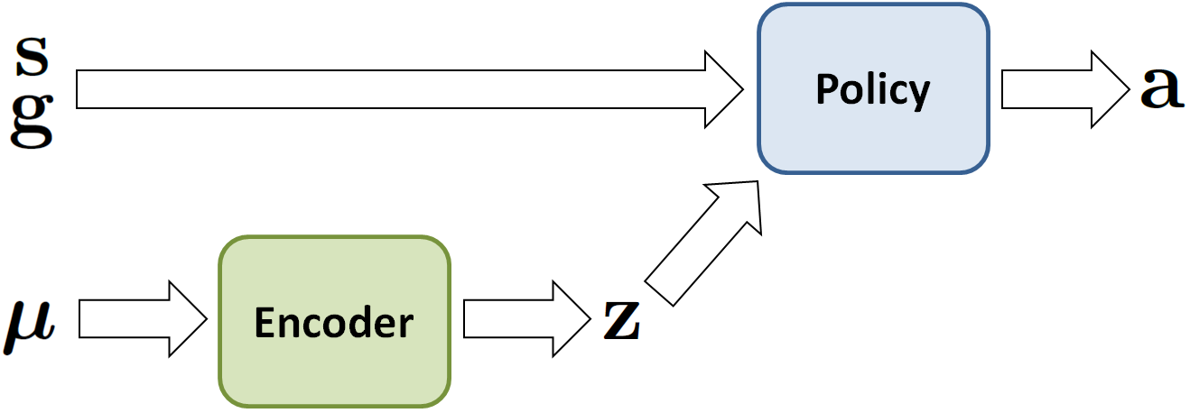
End-to-end deep reinforcement learning without reward engineering


By Avi Singh

Communicating the goal of a task to another person is easy: we can use language, show them an image of the desired outcome, point them to a how-to video, or use some combination of all of these. On the other hand, specifying a task to a robot for reinforcement learning requires substantial effort. Most prior work that has applied deep reinforcement learning to real robots makes uses of specialized sensors to obtain rewards or studies tasks where the robot’s internal sensors can be used to measure reward. For example, using thermal cameras for tracking fluids, or purpose-built computer vision systems for tracking objects. Since such instrumentation needs to be done for any new task that we may wish to learn, it poses a significant bottleneck to widespread adoption of reinforcement learning for robotics, and precludes the use of these methods directly in open-world environments that lack this instrumentation.

We have developed an end-to-end method that allows robots to learn from a modest number of images that depict successful completion of a task, without any manual reward engineering. The robot initiates learning from this information alone (around 80 images), and occasionally queries a user for additional labels. In these queries, the robot shows the user an image and asks for a label to determine whether that image represents successful completion of the task or not. We require a small number of such queries (around 25-75), and using these queries, the robot is able to learn directly in the real world in 1-4 hours of interaction time, resulting in one of the most efficient real-world image-based robotic RL methods. We have open-sourced our implementation.


Our method allows us to solve a host of real world robotics problems from pixels in an end-to-end fashion without any hand-engineered reward functions.

Classifier-based rewards

While most prior work uses purpose-built systems for obtaining rewards to solve the task at hand, a simple alternative has been previously explored. We can specify the task using a set of goal images, and then train a classifier to distinguish between goal and non-goal images. The success probabilities from this classifier can then be used as reward for training an RL agent to achieve the goal.


It’s often straightforward to specify a task via example images. For examples, in the images above, the task could be pour this much wine in the glass, fold clothes like this, and set the table like this.

Problem with classifiers

While classifiers are an intuitive and straightforward solution to specify tasks for RL agents in the real world, they also pose a number of issues when applied to real-world problems. A user that is specifying a task with goal classifiers must provide not only positive examples for the task, but also negative examples. Moreover, this set of negative examples must be exhaustive and cover all parts of the space that the robot can potentially visit. If the set of negative examples is not exhaustive, then the RL algorithm can easily fool the classifier by finding situations that the classifier did not see during training. An example of this classifier exploitation problem can be seen below.


In this task, the goal is to push the green object onto the red marker. The robot is trained via RL using a classifier as a reward function. The success probability from the classifier is visualized with time in the lower right. As we see, while the classifier outputs a success probability of 1.0, the robot does not solve the task. The RL algorithm has managed to exploit the classifier by moving the robot arm in a peculiar way, since the classifier was not trained on this specific kind of negative examples.

Overcoming classifier exploitation

Our recent approach, which we call variational inverse control with events (VICE) seeks to solve this issue by instead mining the negative examples required by the classifier in an adversarial fashion. The method begins by randomly initializing the classifiers and the policy. It first fixes the classifier and updates the policy to maximize the reward. Then, it trains the classifier to distinguish between user-provided goal examples and samples collected by the policy. The RL algorithm then utilizes this updated classifier as reward for learning a policy to achieve the desired goal, and this alternating process continues until the samples collected by the policy are indistinguishable from the user-proved goal examples. This process resembles generative adversarial networks and is based on a form of inverse reinforcement learning, but in contrast to standard inverse reinforcement learning, it does not require example demonstrations – only example success images provided at the beginning of training for the classifier. VICE (as shown below) is effective at combating the exploitation problem faced by naive classifiers, and the user no longer needs to provide any negative examples at all.


We see that the success probabilities learned by the classifier correlate strongly with actual success, allowing the robot to learn a policy that successfully accomplishes the task.

Leveraging active learning

While VICE is capable of learning end-to-end policies for solving real world robotic tasks without any engineering for obtaining rewards, it does have a limitation: it needs thousands of positive examples provided upfront in order to learn, and this could be a burden on the human user. To combat this problem, we developed a new approach that enables the robot to query the user for labels, in addition to using a modest number of initially-provided goal examples. We refer to this approach as reinforcement learning with active goal queries (RAQ). In these active queries, the robot shows the user an image and asks for a label to determine whether the image represents successful completion of the task. While requesting labels for every single state would amount to asking the user to manually provide the reward signal, our method requires labels for only a tiny fraction of the images seen during training, making it an efficient and practical approach for learning skills without manually engineered rewards.


In this task, the goal is to place a book into any one of the empty slots in the bookshelf. This figure shows some example queries made by our algorithm. The algorithm has picked each of these images from the experience it collected while learning to solve the task (using probability estimates from the learned classifier), and the user provides a binary success/failure label for each of them.

The combined method, which we call VICE-RAQ, is able to solve real world robotics tasks with about 80 goal example images provided up front, followed by 25-75 active queries. We make use of the recently introduced soft actor-critic algorithm for policy optimization, and are able to solve tasks in about 1-4 hours of real world interaction time, which is much faster than prior work for a policy trained end-to-end on images.


Our method is able to learn the pushing task (where the goal is to push the mug onto the white coaster) in slightly over an hour of interaction time, and only requires for 25 queries. Even for the more complex bookshelf and draping tasks, our method requires under four hours of interaction time and less than 75 active queries.

Solving tasks involving deformable objects

Since we learn a reward function on pixels, we can solve tasks for which it would be difficult to manually specify a reward function. One of the tasks in our experiments is to drape a cloth over a box, which is essentially a miniaturized version of a tablecloth draping task. To succeed, the robot must drape the cloth smoothly, without crumpling it and without creating any wrinkles. We see that our method is able to successfully solve this task. To demonstrate the challenges associated with this task, we evaluate a method that only uses the robot’s end-effector position as observation and a hand-defined reward function on this observation (Euclidean distance to the goal). We observe that this baseline fails to achieve the objective of this task, as it simply moves the end effector in a straight line motion to the goal, while this task cannot be solved using any straight-line trajectory.


Left: resulting policy with a hand-defined reward on the gripper position. Right: resulting policy from a learned reward function on pixels.

Solving tasks with multiple goal conditions

Classifiers are more expressive than just goal images for describing a task, and this can best be seen in tasks for which there are multiple images that describe our goal. In the bookshelf task in our experiments, the goal is to insert a book into an empty slot on a bookshelf. The initial position of the arm holding the book is randomized, requiring the robot to succeed from any starting position. Crucially, the bookshelf has several open slots, which means that, from different starting positions, different slots may be preferred. Here, we see that our method learns a policy to insert the book in different slots in the bookshelf depending on where the book is at the start of a trajectory. The robot usually prefers to put the book in the nearest slot, since this maximizes the reward that it can obtain from the classifier.


Left: robot chooses to insert book in left slot. Right: robot chooses to insert book in the right slot.

Several data-driven approaches have been proposed for the reward specification problem, and inverse reinforcement learning (IRL) is one of the more prominent frameworks in this setting. VICE is closely related to recent IRL methods like guided cost learning and adversarial inverse reinforcement learning. While these methods require trajectories of (state,action) pairs provided by a human expert, VICE only requires the final desired state, making it substantially easier to specify the task, and also making it possible for the reinforcement learning algorithm to discover novel ways to complete the task on its own (instead of simply mimicking the expert).

Our method is also related to generative adversarial networks. Techniques inspired by GANs have been applied to control problems, but these techniques also require expert trajectories similar to the IRL techniques mentioned before. Our method demonstrates that such adversarial learning frameworks can be extended to settings where we don’t have expert demonstrations, and only have examples of desired states that we would like to achieve.

End-to-end perception and control for robotics have gained prominence in the last few years, but initial approaches either required access to low-dimensional states (e.g. the positions of objects) at training time, or separately trained intermediate representations. More recent approaches are able to learn policies directly on pixels without using low-dimensional states during training, but still require instrumentation for obtaining rewards. Our method goes a step further – it learns both a policy as well as a reward function on pixels. This allows us to solve tasks for which rewards to would be otherwise hard to specify, such as the draping task.

Conclusion

By enabling robotic reinforcement learning without user-programmed reward functions or demonstrations, we believe that our approach represents a significant step towards making reinforcement learning a practical, automated, and readily usable tool for enabling versatile and capable robotic manipulation. By making it possible for robots to improve their skills directly in real-world environments, without any instrumentation or manual reward design, we believe that our method also represents a step toward enabling lifelong learning for robotic systems that learn directly “in the wild”. This capability can make it feasible in the future for robots to acquire broad and highly generalizable skill repertoires directly through interaction with the real world.

This post is based on the following papers:

I would like to thank Sergey Levine, Chelsea Finn and Kristian Hartikainen for their feedback while writing this blog post. This article was initially published on the BAIR blog, and appears here with the authors’ permission.
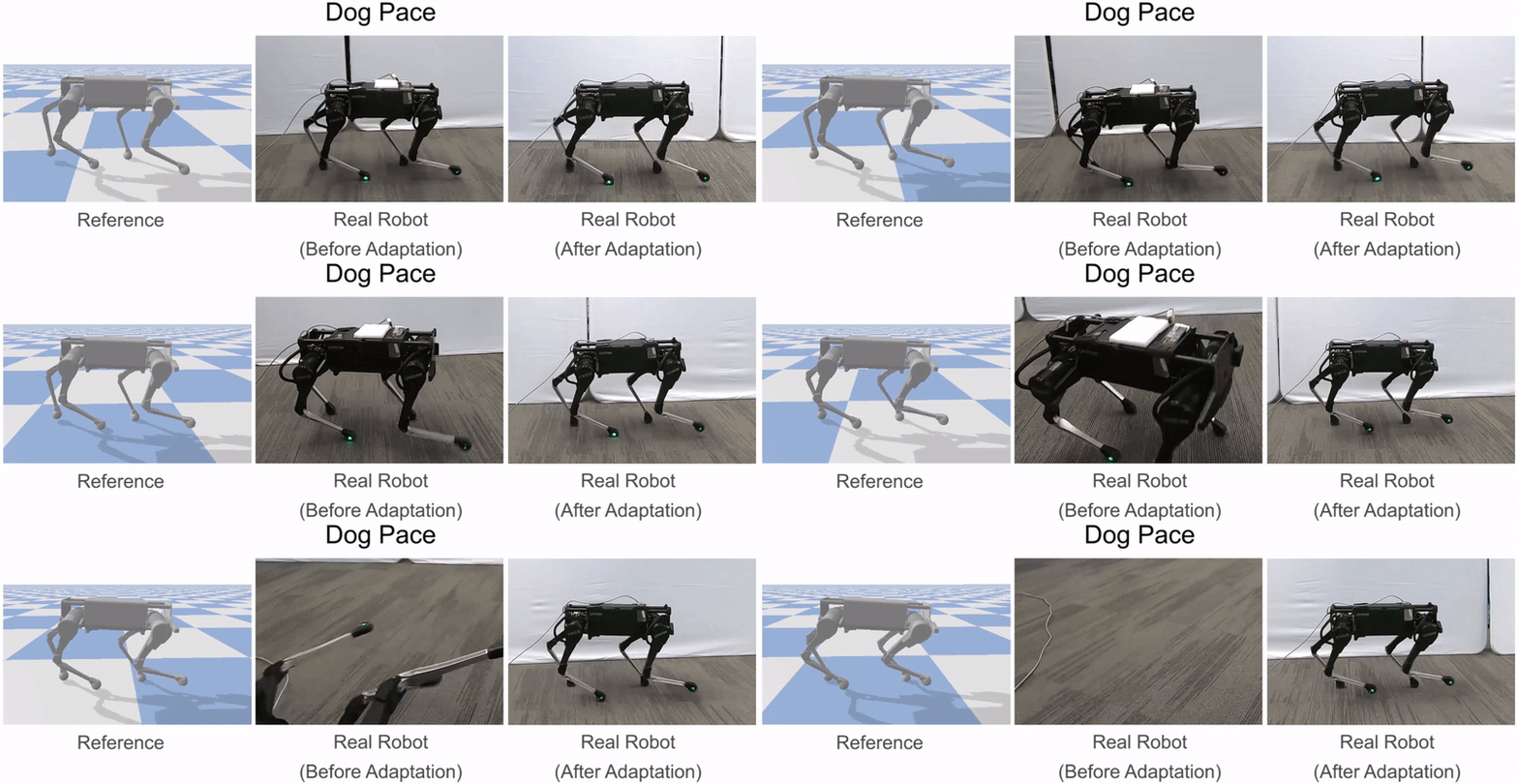
Model-based reinforcement learning from pixels with structured latent variable models

By Marvin Zhang and Sharad Vikram

Imagine a robot trying to learn how to stack blocks and push objects using visual inputs from a camera feed. In order to minimize cost and safety concerns, we want our robot to learn these skills with minimal interaction time, but efficient learning from complex sensory inputs such as images is difficult. This work introduces SOLAR, a new model-based reinforcement learning (RL) method that can learn skills – including manipulation tasks on a real Sawyer robot arm – directly from visual inputs with under an hour of interaction. To our knowledge, SOLAR is the most efficient RL method for solving real world image-based robotics tasks.


Our robot learns to stack a Lego block and push a mug onto a coaster with only inputs from a camera pointed at the robot. Each task takes an hour or less of interaction to learn.

In the RL setting, an agent such as our robot learns from its own experience through trial and error, in order to minimize a cost function corresponding to the task at hand. Many challenging tasks have been solved in recent years by RL methods, but most of these success stories come from model-free RL methods, which typically require substantially more data than model-based methods. However, model-based methods often rely on the ability to accurately predict into the future in order to plan the agent’s actions. This is an issue for image-based learning as predicting future images itself requires large amounts of interaction, which we wish to avoid.

There are some model-based RL methods that do not require accurate future prediction, but these methods typically place stringent assumptions on the state. The LQR-FLM method has been shown to learn new tasks very efficiently, including for real robotic systems, by modeling the dynamics of the state as approximately linear. This assumption, however, is prohibitive for image-based learning, as the dynamics of pixels in a camera feed are far from linear. The question we study in our work is: how can we relax this assumption in order to develop a model-based RL method that can solve image-based tasks without requiring accurate future predictions?

We tackle this problem by learning a latent state representation using deep neural networks. When our agent is faced with images from the task, it can encode the images into their latent representations, which can then be used as the state inputs to LQR-FLM rather than the images themselves. The key insight in SOLAR is that, in addition to learning a compact latent state that accurately captures the objects, we specifically learn a representation that works well with LQR-FLM by encouraging the latent dynamics to be linear. To that end, we introduce a latent variable model that explicitly represents latent linear dynamics, and this model combined with LQR-FLM provides the basis for the SOLAR algorithm.

Stochastic Optimal Control with Latent Representations

SOLAR stands for stochastic optimal control with latent representations, and it is an efficient and general solution for image-based RL settings. The key ideas behind SOLAR are learning latent state representations where linear dynamics are accurate, as well as utilizing a model-based RL method that does not rely on future prediction, which we describe next.

Linear Dynamical Control


Using the system state, LQR-FLM and related methods have been used to successfully learn a myriad of tasks including robotic manipulation and locomotion. We aim to extend these capabilities by automatically learning the state input to LQR-FLM from images.

One of the best-known results in control theory is the linear-quadratic regulator (LQR), a set of equations that provides the optimal control strategy for a system in which the dynamics are linear and the cost is quadratic. Though real world systems are almost never linear, approximations to LQR such as LQR with fitted linear models (LQR-FLM) have been shown to perform well at a variety of robotic control tasks. LQR-FLM has been one of the most efficient RL methods at learning control skills, even compared to other model-based RL methods. This efficiency is enabled by the simplicity of linear models as well as the fact that these models do not need to predict accurately into the future. This makes LQR-FLM an appealing method to build from, however the key limitation of this method is that it normally assumes access to the system state, e.g., the joint configuration of the robot and the positions of objects of interest, which can often be reasonably modeled as approximately linear. We instead work from images and relax this assumption by learning a representation that we can use as the input to LQR-FLM.

Learning Latent States from Images


The graphical model we set up presumes that the images we observe are a function of a latent state, and the states evolve according to linear dynamics modulated by actions, and where the costs are given by a quadratic function of the state and action.

We want our agent to extract, from its visual input, a state representation where the dynamics of the state are as close to linear as possible. To accomplish this, we devise a latent variable model in which the latent states obey linear dynamics, as detailed in the graphic above. The dark nodes are what we observe from interacting with the environment – namely, images, actions taken by the agent, and costs. The light nodes are the underlying states, which is the representation that we wish to learn, and we posit that the next state is a linear function of the current state and action. This model bears strong resemblance to the structured variational auto-encoder (SVAE), a model previously applied to applications such as characterizing videos of mice. The method that we use to fit our model is also based off of the method presented in this prior work.

At a high level, our method learns both the state dynamics and an encoder, which is a function that takes as input the current and past images and outputs a guess of the current state. If we encode many observation sequences corresponding to the agent’s interactions with the environment, we can see if these state sequences behave according to our learned linear dynamics – if they don’t, we adjust our dynamics and our encoder to bring them closer in line. One key aspect of this procedure is that we do not directly optimize our model to be accurate at predicting into the future, since we only fit linear models retrospectively to the agent’s previous interactions. This strongly complements LQR-FLM which, again, does not rely on prediction for good performance. Our paper provides more details about our model learning procedure.

The SOLAR Algorithm


Our robot iteratively interacts with its environment, uses this data to update its model, uses this model to estimate the latent states and their dynamics, and uses these dynamics to update its behavior.

Now that we have described the building blocks of our method, how do these pieces fit together into the SOLAR method? The agent acts in the environment according to its policy, which prescribes actions based on the current latent state estimate. These interactions produce trajectories of images, actions, and costs that are then used to fit the model detailed in the previous section. Afterwards, using these entire trajectories of interactions, our model retrospectively refines its estimate of the latent dynamics, which allows LQR-FLM to produce an updated policy that should perform better at the given task, i.e., incur lower costs. The updated policy is then used to collect more trajectories, and the procedure repeats. The graphic above depicts these stages of the algorithm.

The key difference between LQR-FLM and most other model-based RL methods is that the resulting models are only used for policy improvement and not for prediction into the future. This is useful in settings where the observations are complex and difficult to predict, and we extend this benefit into image-based settings by introducing latent states that we can estimate alongside the dynamics. As seen in the next section, SOLAR can produce good policies for image-based robotic manipulation tasks using only one hour of interaction time with the environment.

Experiments


Left: For Lego block stacking, we experiment with multiple starting positions of the arm and block. For pushing, we only use sparse rewards provided by a human pushing a key when the robot succeeds. Example image observations are given in the bottom row. Right: Examples of successful behaviors learned by SOLAR.

Our main testbed for SOLAR is the Sawyer robotic arm, which has seven degrees of freedom and can be used for a variety of manipulation tasks. We feed the robot images from a camera pointed at its arm and the relevant objects in the scene, and we task our robot with learning Lego block stacking and mug pushing, as detailed below.

Lego Block Stacking

https://youtube.com/watch?v=X5RjE–TUGs%3Frel%3D0

Using SOLAR, our Sawyer robot efficiently learns stacking from only image observations from all three initial positions. The ablations are less successful, and DVF does not learn as quickly as SOLAR. In particular, these methods have difficulty with the challenging setting where the block starts on the table.

The main challenge for block stacking stems from the precision required to succeed, as the robot must very accurately place the block in order to properly connect the pieces. Using SOLAR, the Sawyer learns this precision from only the camera feed, and moreover the robot can successfully learn to stack from a number of starting configurations of the arm and block. In particular, the configuration where the block starts on the table is the most challenging, as the Sawyer must learn to first lift the block off the table before stacking it – in other words, it can’t be “greedy” and simply move toward the other block.

We first compare SOLAR to an ablation that uses a standard variational auto-encoder (VAE) rather than the SVAE, which means that the state representation is not learned to follow linear dynamics. This ablation is only successful on the easiest starting configuration. In order to understand what benefits we extract from not requiring accurate future predictions, we compare to another ablation which replaces LQR-FLM with an alternative planning method known as model-predictive control (MPC), and we also compare to a state-of-the-art prior method that uses MPC, deep visual foresight (DVF). MPC has been used in a number of prior and subsequent works, and it relies on being able to generate accurate future predictions using the learned model in order to determine what actions are likely to lead to good performance.

The MPC ablation learns more quickly on the two easier configurations, however, it fails in the most difficult setting because MPC greedily reduces the distance between the two blocks rather than lifting the block off the table. MPC acts greedily because it only plans over a short horizon, as predicting future images becomes increasingly inaccurate over longer horizons, and this is exactly the failure mode that SOLAR is able to overcome by utilizing LQR-FLM to avoid future predictions altogether. Finally, we find that DVF can make progress but ultimately is not able to solve the two harder settings even with more data than what we use for our method. This highlights our method’s data efficiency, as we use in total a few hours of robot data compared to days or weeks of data as in DVF.

Mug Pushing

https://youtube.com/watch?v=buk4YE2mFTs%3Frel%3D0

Despite the challenge of only having sparse rewards provided by a human key press, our robot running SOLAR learns to push the mug onto the coaster in under an hour. DVF is again not as efficient and does not learn as quickly as SOLAR.

We add an additional challenge to mug pushing by replacing the costs with a sparse reward signal, i.e., the robot only gets told when it has completed the task, and it is told nothing otherwise. As seen in the picture above, the human presses a key on the keyboard in order to provide the sparse reward, and the robot must reason about how improve its behavior in order to achieve this reward. This is implemented via a straightforward extension to SOLAR, as we detail in the paper. Despite this additional challenge, our method learns a successful policy in about an hour of interaction time, whereas DVF performs worse than our method using a comparable amount of data.

Simulated Comparisons


Left: an illustration of the car and reacher environments we experiment with, along with example image observations in the bottom row. Right: our method generally performs better than the ablations we compare to, as well as RCE. PPO has better final performance, however PPO requires one to three orders of magnitude more data than SOLAR to reach this performance.

In addition to the Sawyer experiments, we also run several comparisons in simulation, as most prior work does not experiment with real robots. In particular, we set up a 2D navigation domain where the underlying system actually has linear dynamics and quadratic cost, but we can only observe images that show a top-down view of the agent and the goal. We also include two domains that are more complex: a car that must drive from the bottom right to the top left of a 2D plane, and a 2 degree of freedom arm that is tasked with reaching to a goal in the bottom left. All domains are learned with only image observations that provide a top down view of the task.

We compare to robust locally-linear controllable embeddings (RCE), which takes a different approach to learning latent state representations that follow linear dynamics. We also compare to proximal policy optimization (PPO), a model-free RL method that has been used to solve a number of simulated robotics domains but is not data efficient enough for real world learning. We find that SOLAR learns faster and achieves better final performance than RCE. PPO typically learns better final performance than SOLAR, but this typically requires one to three orders of magnitude more data, which again is prohibitive for most real world learning tasks. This kind of tradeoff is typical: model-free methods tend to achieve better final performance, but model-based methods learn much faster. Videos of the experiments can be viewed on our project website.

Related Work

Approaches to learning latent representations of images have proposed objectives such as reconstructing the image and predicting future images. These objectives do not line up perfectly with our objective of accomplishing tasks – for example, a robot tasked with sorting objects into bins by color does not need to perfectly reconstruct the color of the wall in front of it. There has also been work on learning state representations that are suitable for control, including identifying points of interest within the image and learning latent states such that dimensions are independently controllable. A recent survey paper categorizes the landscape of state representation learning.

Separately from control, there has been a number of recent works that learn structured representations of data, many of which extend VAEs. The SVAE is an example of one such framework, and some other methods also attempt to explain the data with linear dynamics. Beyond this, there have been works that learn latent representations with mixture model structure, various discrete structures, and Bayesian nonparametric structures.

Ideas that are closely related to ours have been proposed in prior and subsequent work. As mentioned before, DVF has also learned robotics tasks directly from vision, and a recent blog post summarizes their results. Embed to control and its successor RCE also aim to learn latent state representations with linear dynamics. We compare to these methods in our paper and demonstrate that our method tends to exhibit better performance. Subsequent to our work, PlaNet learns latent state representations with a mixture of deterministic and stochastic variables and uses them in conjunction with MPC, one of the baseline methods in our evaluation, demonstrating good results on several simulated tasks. As shown by our experiments, LQR-FLM and MPC each have their respective strengths and weaknesses, and we found that LQR-FLM was typically more successful for robotic control, avoiding the greedy behavior of MPC.

Future Work

We see several exciting directions for future work, and we’ll briefly mention two. First, we want our robots to be able to learn complex, multi-stage tasks, such as building Lego structures rather than just stacking one block, or setting a table rather than just pushing one mug. One way we may realize this is by providing intermediate images of the goals we want the robot to accomplish, and if we expect that the robot can learn each stage separately, it may be able to string these policies together into more complex and interesting behaviors. Second, humans don’t just learn representations of states but also actions – we don’t think about individual muscle movements, we group such movements together into “macro-actions” to perform highly coordinated and sophisticated behaviors. If we can similarly learn action representations, we can enable our robots to more efficiently learn how to use hardware such as dexterous hands, which will further increase their ability to handle complex, real-world environments.

This post is based on the following paper:

We would like to thank our co-authors, without whom this work would not be possible, for also contributing to and providing feedback on this post, in particular Sergey Levine. We would also like to thank the many people that have provided insightful discussions, helpful suggestions, and constructive reviews that have shaped this work. This article was initially published on the BAIR blog, and appears here with the authors’ permission.
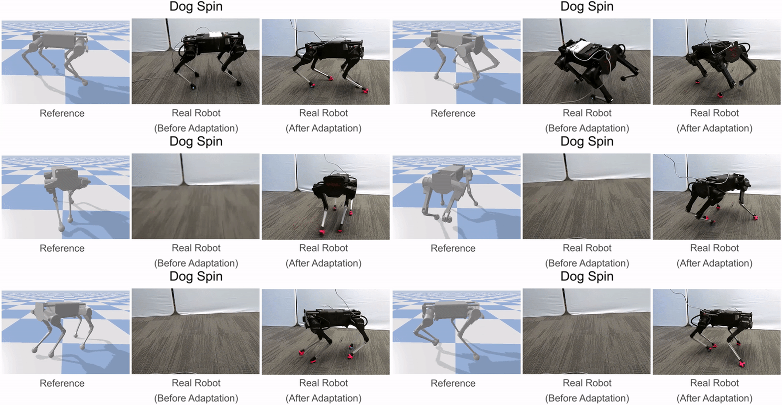
Page 2 of 4
1 2 3 4